


Lesson one: Introduction to HETVAL Subroutine in ABAQUS
What is the purpose of developing the HETVAL subroutine?
The first lesson begins by explaining the primary reason for the development of the HETVAL subroutine. In the first section of this lesson, we will discuss what the HETVAL subroutine is and why it is provided. Then, we will explore various applications of HETVAL, demonstrating its usefulness. These applications may include simulating heat generation in phase change materials, modeling the heat generated due to chemical reactions, and analyzing the thermal behavior of metal alloys and composite materials. After exploring the subroutine’s applications, for those who may not be familiar with Abaqus subroutines, we will explain how HETVAL links to Abaqus and how it works.
How to use the HETVAL subroutine?
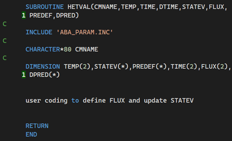
The primary question is how to utilize the HETVAL subroutine, a topic explored in the second section. In this section, we initially discuss the conditions under which the subroutine can be employed. Next, we provide information on the location of its documentation and how to access it, especially for those who prefer reviewing it themselves. Additionally, we cover the required settings that need to be defined within Abaqus to enable the reading of heat flux from the subroutine. These settings must be applied to material properties in Abaqus. The main part of the lesson starts here, where we introduce the subroutine interface. Following the introduction to this interface, you will acquire a fundamental understanding of the process for writing the subroutine.
What are the subroutine variables?
In the third section, we will discuss the subroutine variables. The first group includes variables passed in for information, such as time, temperature, field variables, and the material name. Then, we will cover the variables that need to be defined within the subroutine to be sent to Abaqus, such as heat flux. Finally, we will introduce variables that can be updated during the solution if needed, such as state variables. We will delve into detailed discussions of these variables in this section. After that, you will gain an understanding of the subroutine’s variables. However, to use the subroutine effectively, we also need to define certain material properties such as density and specific heat capacity in Abaqus, which we will discuss towards the end of this section. By the end of this section, you will be prepared to begin using HETVAL to solve numerical examples.
Workshop 1
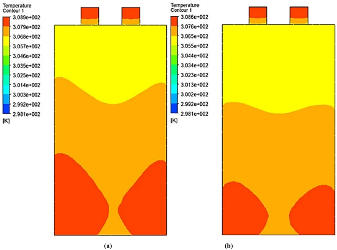
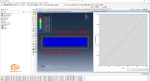
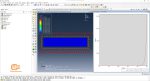
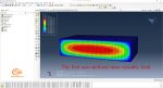
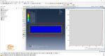
The first workshop involves exploring a straightforward 2D plate subjected to constant heat flux, as outlined in the Abaqus documentation. This example is very simple, chosen specifically to demonstrate how the subroutine can be applied to such a particular problem. Moreover, a step-by-step guide is provided to demonstrate how you can model the problem in Abaqus. Our goal is to extract the domain temperature influenced by the heat flux and then compare it with reference results for verification purposes.
Workshop 2
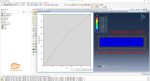
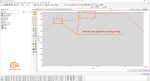
The second workshop builds upon the problem addressed in the first workshop by introducing a more complex heat flux scenario. The workshop aims to illustrate how the subroutine operates within a scenario where the heat flux varies with time, a common occurrence in many realistic problems. In this context, we will utilize time as an input parameter in the subroutine to calculate the varying heat flux. Following this approach, we have solved the problem and compared the obtained results with an analytical solution to verify their accuracy.
Workshop 3
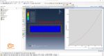
In many practical applications, the heat flux is a function of the current temperature and varies accordingly. To demonstrate how the subroutine addresses such scenarios, we have introduced the third workshop. In this workshop, we revisit the problem addressed in the previous workshops but with a different heat flux condition. Here, the heat flux is a function of temperature. It is important to note that this subroutine is more complex than those in the previous workshops; because when the heat flux depends on temperature, the subroutine also needs to calculate the variation of heat flux concerning time, a calculation that is performed in this workshop. We have solved the problem and verified the results to ensure the accuracy of our solution.
Workshop 4
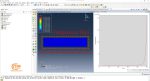
A powerful capability of the subroutine is its ability to define the heat flux as a function of user-defined state variables. During the solution, we can call upon these state variables, update them, and retain their values for the subsequent calls. This capability enables the solution of various problems involving factors such as damage, cure degree, or other related parameters. To demonstrate how to address such problems, we have explored this capability in the fourth workshop. In this workshop, we have revisited the problem in the previous workshops, but with the distinction that the heat flux is dependent on the state variables. We solved the problem and verified the results to ensure the accuracy and validity of the procedure.
Workshop 5
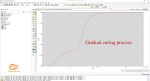
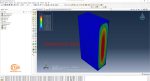
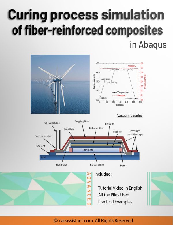
The last workshop is significantly more complex compared to the previous ones, as it explores a practical scenario to demonstrate how HETVAL can be applied to a realistic problem. In this workshop, we will simulate the curing process in fiber-reinforced composite laminates, an essential step before these laminates can be utilized in the industry. The curing process involves applying heat to meet industry standards for the composite, making it a crucial step in fiber-reinforced composite production. Numerical simulation of this process is challenging and necessitates a thermochemical coupled model to compute the heat released from chemical reactions during curing. Workshop 5 offers a step-by-step guide on simulating the curing process using Abaqus with HETVAL to simplify this complex process.
Lesson 2: Simulation of the Curing Process in Fiber-Reinforced Composites
We hope you have learned everything you expected from Lesson 1 and its workshops. However, upon exploring Workshop 5, you might ask questions like, ‘What is the curing process in fiber-reinforced composites?’ or even, ‘What are fiber-reinforced composites, and where are they used?’. We have answered these questions in the second lesson, which consists of five sections.
What are fiber-reinforced composites (FRCs)?
In the first section of the second lesson, we will discuss what are fiber-reinforced composites. A fiber-reinforced composite comprises two distinct constituents: fibers and a matrix. The fibers offer exceptional strength and stiffness and take up most of the load applied to the composite. On the other hand, the matrix functions as a cohesive agent, binding the fibers together, contributing to distributing the load among the fibers, protecting them from damage, and ensuring the overall structural consistency of the composite. This mixture leads to a material that demonstrates superior properties compared to each component on its own.
Fiber-reinforced composites are recognized for their lightweight characteristics, durability, and strength, making them highly advantageous in a wide range of industries. Based on such specifications, they can be utilized across multiple fields such as aerospace, automotive, construction, sports equipment, and beyond. Due to their outstanding qualities, FRCs have become one of the most promising materials in modern times.
FRCs can be classified into different categories based on the materials they incorporate. Common matrix types include polymers, metals, or ceramics, with a specific focus on polymers in this context. Additionally, composite materials differ based on the fibers used, frequently including materials like glass, carbon, and aramid. They can suffer from diverse configurations, including single or multiple layers, and possess either unidirectional or multidirectional properties, customized for particular purposes. The diverse range of compositions leads to a multitude of behaviors and applications across multiple industries.
How FRCs are made?
Regardless of their classification, modern composites are frequently produced employing two techniques: Resin Transfer Molding (RTM) and Prepreg. Each technique has specific advantages. RTM involves injecting resin into a mold, which is filled with dry reinforcing fibers. The resin injection, conducted under pressure, helps remove air and thoroughly saturate the fibers. Subsequently, the mold undergoes heating to assist in the curing of the resin.
On the other hand, Prepreg consists of reinforcing fibers embedded in a controlled environment within a resin matrix. The resin is partially cured but not fully solidified. During the manufacturing process, these prepreg sheets are placed into molds and undergo further curing under heat and pressure to achieve the final product. This method ensures precise control over resin levels, resulting in consistent final composites that produce high-quality components with exceptional mechanical properties.
Although both techniques use resin and fiber reinforcement, the key distinction lies in how the resin is employed. In both methods, the composite undergoes cycles of pressure and temperature to transform the resin from a liquid to a solid state. This critical process, referred to as curing, is essential for all applications and demands careful accuracy.
Two primary methods are commonly employed to apply heat and pressure to cure composite materials: oven heating and autoclave curing. The autoclave method, although more advanced and precise, comes with a higher cost. Whether utilizing an oven or an autoclave, the curing process requires careful planning to maintain the composite’s performance and quality, while also improving its surface finish. Hence, the curing process plays a critical role in the manufacturing of FRCs.
Simulating the curing process in FRCs
Time and temperature are fundamental elements that impact the curing quality of fiber-reinforced composites. High-quality composites often necessitate several hours of curing at an ideal temperature to meet industry standards. However, this extended curing duration can slow down production and decrease efficiency. As a result, many manufacturers opt for shorter curing periods at higher temperatures to boost production rates. However, this strategy might induce residual stress in the composite, affecting its overall quality. Hence, it becomes crucial to optimize the curing process to strike a balance between quality and time. Numerical simulation emerges as a cost-effective method to achieve this optimization.
In simulating the curing process, the degree of cure stands as a crucial parameter that dictates how extensively the material is cured. This degree is influenced by how heat spreads within the material. The complexity arises from having two sources of heat: external heat and internal heat resulting from chemical reactions within the matrix. The internal heat is related to the degree of cure. Hence, studying this behavior demands a thermo-chemical model. Furthermore, the overall strain includes mechanical strains, curing shrinkage strains, and thermal expansion. Therefore, an accurate prediction of stress and strain fields requires a thermo-mechanical model.
The thermochemical model needs to include both a heat transfer equation and a cure kinetic equation to precisely describe the curing process. Within the cure kinetic equation, the curing rate dictates the heat flux, and this rate varies according to the particular composite material being used. Consequently, a single equation cannot be universally applied to all materials. Nonetheless, the existing thermochemical models involve the Fourier heat conduction law and the energy balance law. Please note that for the sake of simplicity within this package, we have omitted the mechanical field during curing. So, only the heat release resulting from chemical reactions is considered.
How simulation is conducted in this lesson
The thermochemical model is variable and not universally standardized due to differences in composite properties. Therefore, exploring all these models into a single lesson is not feasible. However, within this lesson, we have chosen a well-known composite type: AS4/3501–6 multidirectional carbon/epoxy prepreg for simulation. Here, we will explain the thermochemical model tailored specifically for simulating this particular material. The model will play a role in simulating the curing process and extracting parameters like the degree of cure and temperature distribution within the composite. Abaqus, equipped with the HETVAL subroutine, will be employed to define and implement the model.
Required subroutines in this lesson
Due to the complexity of curing problems, depending solely on Abaqus for simulations is insufficient. To overcome this limitation, we have integrated Abaqus subroutines into our approach. For instance, the HETVAL subroutine manages heat flux produced by chemical reactions, and DISP defines curing cycles. Through the utilization of these subroutines, we can simulate complex problems within the Abaqus framework. Furthermore, by learning the provided lessons in this package, you will acquire essential knowledge for writing such subroutines.


lemon skunk –
Love sees no faults.