
Introduction to Finite Element Method | Finite Element Analysis

Ever wondered how engineers predict how bridges bend, planes flex, or heat flows through engines? Solving these real-world problems by hand would be almost impossible — and that’s where the Finite Element Method (FEM) comes in.
The Finite Element Method (FEM) is a powerful numerical tool that breaks complex problems into smaller, solvable pieces.
FEM is a powerful numerical technique used to solve complex engineering and physics problems. Instead of trying to tackle an entire complicated structure at once, FEM breaks it down into many small, manageable pieces called elements. This method is widely used across fields like structural analysis, heat transfer, fluid dynamics, mass transport, and electromagnetics.
Engineers rely on FEM especially when traditional analytical methods fall short — for example, when dealing with:
-
Intricate geometries (like crash simulations),
-
Complex loading conditions (such as time-dependent forces),
-
Advanced material behaviors (like fiber-reinforced plastics or hyperelastic materials).
Thanks to FEM, engineers can model, simulate, and predict the behavior of structures and materials that would otherwise be too difficult or costly to study physically.
👉 Stay with us through this post to discover:
-
What FEM and finite element analysis (FEA) really are,
-
Where they’re applied,
-
And how you can start learning to work with them yourself!

What is included in this package?
Video
5 Workshops
Theory &
Practice
Files
1. What is Finite Element Method (FEM), Really?
In simple terms, FEM is a numerical technique for solving complex problems in physics and engineering. Instead of solving differential equations directly — which is often impossible for real-world structures with complicated shapes, loading conditions, and material properties — FEM approximates the solution numerically.
The finite element approach is widely used in many fields, including:
-
Structural analysis (e.g., bridges, buildings),
-
Heat transfer analysis (e.g., electronics cooling),
-
Fluid flow (e.g., airflow over a car),
-
Mass transport (e.g., chemical diffusion),
-
Electromagnetic potential (e.g., antennas, motors).
FEM is not only limited to engineering and scientific fields but can make it easier for us to solve all life issues. Here are some interesting applications of FEM:
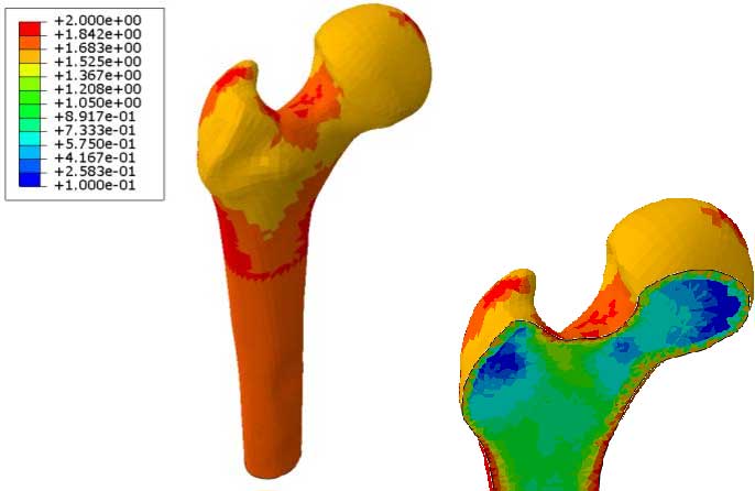 Stress analysis in bone [Ref ] Stress analysis in bone [Ref ] |
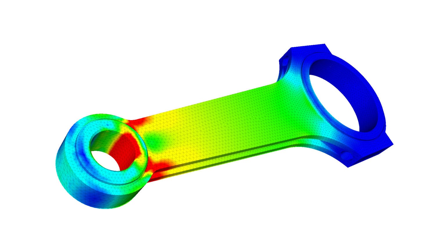
Piston rod analysis [Ref] |
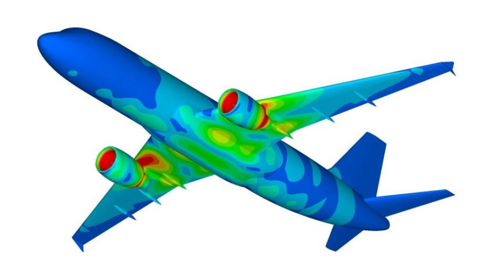
Full scale aircraft analysis[Ref] |
The challenge with these problems is that they involve differential equations that, due to complexity, cannot be solved exactly. Complex geometries, varying forces, and non-uniform materials make it impossible to find neat mathematical solutions.
That’s where numerical techniques like FEM come in.
Instead of solving one big difficult equation, FEM breaks the problem into many small, simple parts (called elements) connected at points (called nodes). This transforms the original complex problem into a large set of simultaneous algebraic equations, which are much easier for computers to solve.
🔵 Think of it like this:
“Instead of trying to understand the structure of a cookie all at once, FEM breaks it into many small crumbs, analyzes each crumb carefully, and then puts the whole picture together.”
Finally, a quick note:
While FEM refers to the mathematical approach, FEA (Finite Element Analysis) is the actual application of FEM to a real-world problem. (We’ll explain more about this difference later — stay tuned!)
2. Why Do We Need the Finite Element Method (FEM)?
In the real world, engineering problems are rarely simple.
Imagine trying to manually calculate the stress in an entire airplane wing, predict the temperature distribution in an engine block, or simulate how blood flows through arteries. These systems are complex — often too complex for traditional hand calculations or simple formulas.
Let me be more academic:
In theory, many physical problems — like how a beam bends under a load or how heat spreads through a metal plate — can be described using differential equations.
But in real life, those equations quickly become impossible to solve exactly when things get complicated.
Here’s why we need FEM:
1. Complex Geometries
Most real-world objects — like car bodies, aircraft wings, or smartphone casings — have irregular, complicated shapes. Solving mathematical equations for these shapes analytically is almost impossible.
FEM handles this complexity by breaking the geometry into many small, simple elements (like triangles, squares, or tetrahedrons) that approximate the real shape.
2. Complex Loading and Boundary Conditions
Real-life forces aren’t always steady or simple.
Loads may change over time, vary in direction, or impact different points simultaneously (think of a car crash simulation or a vibrating turbine blade).
FEM allows engineers to model and analyze these complicated loading conditions with precision.
3. Complex Material Behaviors
Materials in engineering aren’t always simple metals or plastics.
We often deal with:
-
Anisotropic materials (properties differ by direction, like in composites),
-
Inhomogeneous materials (properties vary across the structure),
-
Nonlinear materials (like hyperelastic rubber or plastic deformation).
Analytical methods struggle here — but FEM easily adapts to these complicated material behaviors.
4. Multi-Physics Problems:
Many real problems involve more than one type of physics happening at once, like temperature affecting structural strength, or electric currents influencing fluid flow.
5. Simulations Save Time, Money, and Lives
Instead of building multiple prototypes and running physical experiments (which can be expensive and dangerous), engineers can simulate a product digitally first.
This means:
-
Faster design iterations,
-
Lower development costs,
-
Safer products.
Without FEM, modern industries like automotive, aerospace, and biomedical engineering could not operate at the speed and safety levels we expect today.
FEM doesn’t try to solve the impossible equation all at once.
Instead, it divides the problem into small pieces (elements), approximates the behavior in each piece with simple equations, and then assembles the pieces together to model the whole system.
This allows engineers to:
-
Predict stress and deformation in structures,
-
Simulate temperature distribution in engines,
-
Model fluid flow through pipes and air around vehicles,
-
Analyze electromagnetic fields in devices like MRI machines or electric motors.
Without FEM, many of the advanced designs we see today — from lightweight aircraft to efficient electric cars to safe skyscrapers — would simply not be possible.
👉 In short, FEM bridges the gap between beautiful theory and messy real-world complexity.
📌 Recap:
-
Problem: Real-world systems are too messy for simple math.
-
Solution: FEM breaks problems down into manageable chunks.
-
Result: Engineers can simulate, predict, and improve designs with high accuracy.
3. How Does the Finite Element Method (FEM) Work? | Step-by-Step Guide
At first glance, the Finite Element Method (FEM) may seem complicated, but if we break it down into simple steps, the logic behind it becomes clear and intuitive.
FEM is like solving a huge puzzle: you divide a big problem into smaller parts, understand how each part behaves, and then put them all back together to find the full solution.
Here’s a quick overview of the general FEM process:
| Step | What Happens | Why It's Important |
|---|---|---|
| 1 | Discretize the domain and select element types | Break complex shapes into small, simple parts |
| 2 | Select the U function (degrees of freedom) | Define what you're solving for (displacements, temperature, etc.) |
| 3 | Establish strain-displacement and stress-strain relationships | Connect physics laws to your model |
| 4 | Derive element stiffness matrices and equations | Build the small mathematical model for each element |
| 5 | Assemble global equations and apply boundary conditions | Create and constrain the full system |
| 6 | Solve for unknown degrees of freedom | Find primary solutions (like displacements) |
| 7 | Calculate element strains and stresses | Extract secondary results (stress, strain, etc.) |
| 8 | Analyze and interpret the results | Make real-world engineering decisions |
Now, let’s dive deeper into each step — imagine you’re solving a real-world engineering problem!
3.1. Step 1: Discretize and Select the Element Types
Before we can solve a problem using FEM, we need to break it down into manageable pieces.
This process is called discretization.
In the context of FEM, discretization means dividing a complex structure or domain into a finite number of smaller, simpler parts called elements.
Each of these elements is connected to neighboring elements through points called nodes.
A node is a specific point in space used to define the system’s behavior.
At each node, we assign degrees of freedom (DOFs) — these represent the possible ways the node can move or react under loading (such as translations, rotations, or other physical quantities depending on the problem).
The DOFs are also responsible for transmitting forces, moments, or other effects between the elements.
The practical implementation of discretization is called meshing.
Meshing is the process of generating a network of elements and nodes over the structure’s geometry.
Choosing the right type of element (for example, triangles for 2D problems, tetrahedrons for 3D problems) and the appropriate mesh size is critical.
A finer mesh usually leads to more accurate results, but it also increases computational cost.
🔹 Key takeaway:
Discretization simplifies a complex geometry into smaller parts (elements) connected at points (nodes) with defined degrees of freedom, and meshing brings this idea to life by actually creating the finite element model.
You can see an example in figure 1.
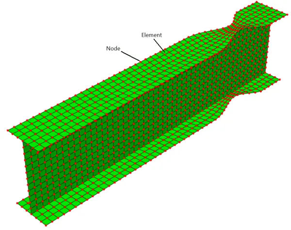
Figure 1: Dividing structure into elements
3.1.1. Element shape function
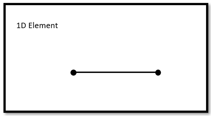
In the FEM engineering, continuous models are estimated using the data from a finite number of discrete locations. Discretization is the process of breaking the structure down into discrete parts. The function that interpolates the solution between the discrete values obtained at the element nodes is known as the shape function. We can choose different element shape functions:
- Line element(1D)
A linear shape function describes a linear element or a lower-order element.
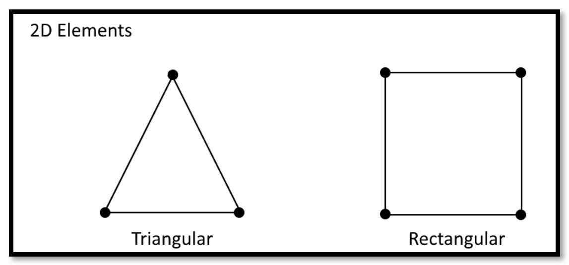
- surface element(2D)
Three or four corner nodes and a part’s mid-surface make up a surface element. The surface thickness must be assigned once it has been developed for the FEA software.
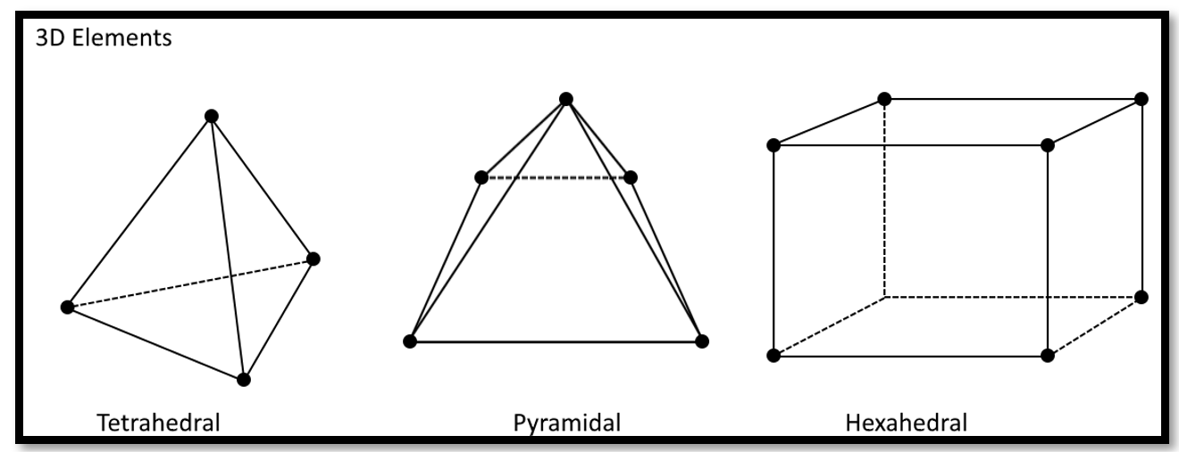
- Solid element(3D)
Since they can be applied to any CAD solid model, solid elements are the most common element type employed by automatic mesh generators in FEA software.
3.1.2. Linear and Higher-Order Elements
The most typical element types were already covered, so I’ll just conclude here. I simply want to make a few things clear in FEM engineering because, regrettably, the names can be a little confusing.
People commonly refer to the “first-order” elements—those that only have Nodes in “corners”—by this name (Shown on the left side of figure 2). And there is another type, typically referred to as quadratic. These components would be considered second-order because in the midst of each of those are extra nodes (Shown on the right side of figure 2).
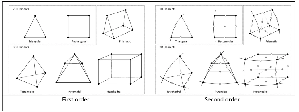
Figure 2: First-order and second-order elements [Ref]
3.2. Step 2: Select U Function (degrees of freedom)
Once the structure is discretized into elements and nodes, the next step is to define how the structure can move.
This is done by selecting a function that describes the system’s possible displacements — called the U function.
First, let’s talk about Degrees of Freedom (DOFs).
Degree of Freedom (DOF) refers to the “ability” to move in a specific direction.
In 3D space, there are six DOFs: translation along the X, Y, and Z axes, and rotation about those same three axes.
These DOFs define the ways a point (node) can move under load.
In FEM, DOFs are essential because they:
-
Control boundary conditions (restrictions of movement)
-
Allow calculation of stresses and internal forces
-
Define how the structure will respond to loads
The concept of DOF appears in many fields — statistics, mechanical systems, robotics, vibrations, and of course, finite element analysis.
For structural problems (like the one we’re focusing on in this article), the primary unknown is usually the displacement of the nodes.
So, in this step, we select a displacement function for each element.
This function approximates the displacement field within each element, based on the nodal values.
For example:
-
In a 2D beam analysis, each node may have three DOFs: translation along the X and Y directions and rotation about the Z-axis.
-
For a single beam element connecting two nodes, we would have six DOFs in total (three per node).
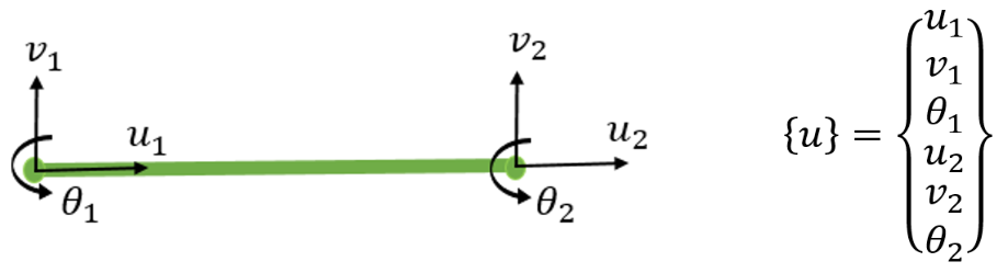
Figure 3: Degrees of freedom for 2D beam element
The displacement function is usually chosen to be a simple polynomial (such as linear or quadratic) that satisfies basic requirements for compatibility and continuity between elements.
By piecing together these simple functions for all elements, FEM approximates the continuous displacement field across the entire structure.
🔹 Key takeaway:
In Step 2, we define how each element can deform by selecting a displacement function based on the degrees of freedom at each node.
Note: there are more to know about elements in Abaqus. You can have them all just by reading the article “Abaqus element types“.
3.2.1. Fundamental Boundary Conditions in FE
Boundary conditions (BCs) are essential constraints for solving boundary value problems, which involve differential equations defined within a domain and governed by known conditions at the boundaries. Unlike initial value problems, where conditions are specified at one end of an interval, boundary value problems are vital for modeling a wide range of phenomena, including solid mechanics, heat transfer, fluid dynamics, and acoustics.
Boundary conditions in continuous systems are generally classified into two categories:
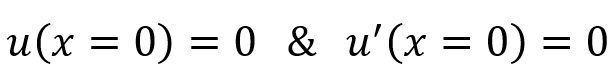
- Geometric (Essential) Boundary Conditions
Also called kinematic BCs, these are dictated by geometric constraints, such as fixing one end of a beam or restricting a shaft’s motion. In FEA tools, these are typically implemented as “fixed BCs.” For example:
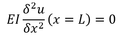
- Force (Natural) Boundary Conditions
Also known as static BCs, these arise from force and moment balances. For example, applying a moment at a cantilever’s free end. These BCs are defined by loads acting on the structure and are crucial for accurate simulations. For example:
3.3. Step 3: Determination of strain/displacement and stress/strain relationships
After discretizing the structure and selecting displacement functions, the next step is to connect these displacements to physical quantities like strain and stress.
First, we need the strain-displacement relationship.
For example, for one-dimensional deformation in the x direction, the strain “εx” is associated with the displacement u by εx=du/dx if the strain is small. Furthermore, stress must be related to strain by the stress-strain law, commonly known as the law of materials. The ability to accurately define material behavior is paramount to achieving acceptable results. Hooke’s law is the simplest of the stress/strain laws and is commonly used in stress analysis.
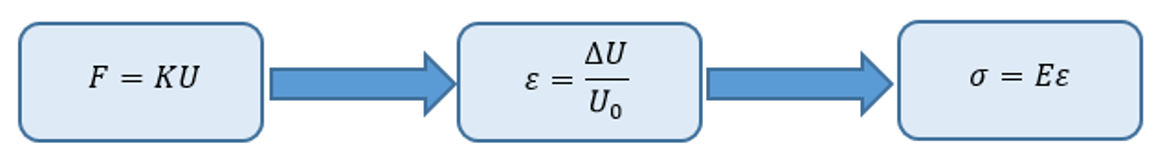
- F: External force
- K: stiffness matrix of element
- U: displacement of each element
- ε: strain of each element
- σ: stress of each element
- E: Young modulus of material
As we said, the example we are considering for this article is about a structural type, and therefore all the written equations are related to the calculation of the stress and strain of the structure. If we want to start our simulation FEA on another subject, we must write the governing equations specific to the new subject. For example, for heat transfer, we have:
Q = CT
Q is proportional to the temperature difference between the objects and the heat capacity C of the object.
🔵 Side Note:
In more advanced FEM studies, nonlinear material models (like plasticity or hyperelasticity) are also used to simulate permanent deformations or rubber-like behaviors.
🔹 Key takeaway:
In Step 3, we establish how displacements create strains and how those strains produce stresses, based on the chosen material model.
You can see the general usage of the FEM and the equation “F=KU” in lesson 2 of the Abaqus course for beginners package. Just go to the “General Usage of FEM” section of this lesson to learn more.
3.4. Step 4: Derive the Element Stiffness Matrix and Equations
In this step, we translate the physical behavior of each element into a mathematical form — specifically into the element stiffness matrix.
The stiffness matrix describes how the element resists deformation when subjected to forces.
It captures the relationship between the nodal forces applied to the element and the resulting nodal displacements.
🔹 Key takeaway:
In Step 4, we create a mathematical model (stiffness matrix) that defines how each element deforms under applied forces.
The development of the element stiffness matrix and element equations is initially based on the concept of factors affecting stiffness, which requires a background in statics. We present an alternative method.
3.4.1. Direct equilibrium Method
According to this method, the stiffness matrix and element equations, which relate nodal forces to nodal displacements, are attained using force equilibrium conditions and force/deformation connections for a basic element. This method is most easily adaptable to line or one-dimensional elements.
What is included in this package?
Video
5 Workshops
Theory &
Practice
Files
For example, to calculate the horizontal displacement of the beam, the following equation can be written:
Now, if these equations are placed next to the boundary conditions, they get a strong form. The strong mode can be used to solve simple elements.

3.4.2. Work or energy Methods
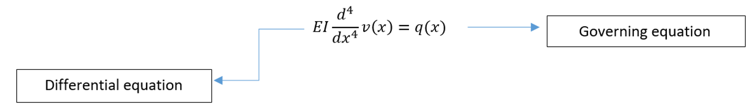
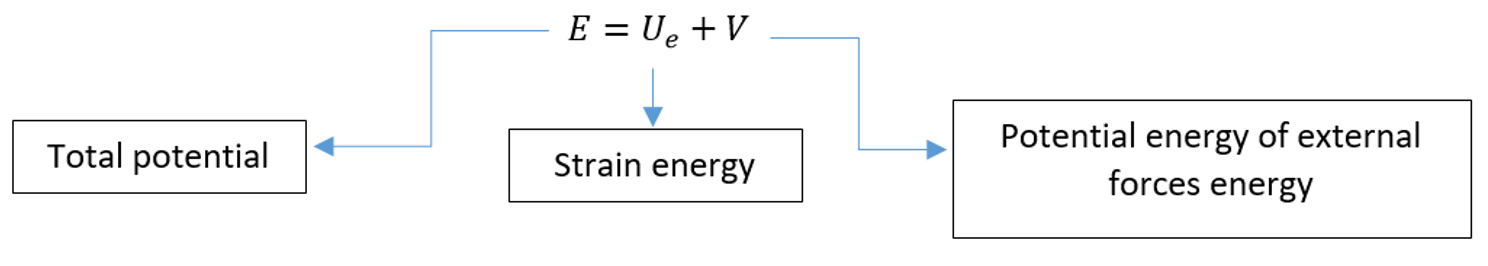
It is much easier to use a work or energy method to develop the stiffness matrix and equations for two- and three-dimensional elements. The principle of virtual work (using virtual displacements), the principle of minimum potential energy, and Castigliano’s theorem are frequently used to derive element equations.
Furthermore, the virtual work principle can be applied even when a potential function does not exist.
Following that, the principle is commonly used to derive all other stress-analysis stiffness matrices and element equations.
A functional similar to the one used with the principle of minimum potential energy is quite useful in deriving the element stiffness matrix and equations to extend the finite element method for the structural stress analysis field.
A functional is an integral expression that implicitly contains differential equations that describe the problem. A typical functional is of the form ![]() where u(x).x and F are real so that I(u) is also a real number. Here
where u(x).x and F are real so that I(u) is also a real number. Here ![]() .
.
We can write this equation for structural analysis:
3.4.3. Weighted residuals Methods
Weighted residual methods, particularly Galerkin’s method, are useful for developing element equations. Wherever energy methods are applicable, these methods produce the same results as energy methods. They are especially useful when a function, such as potential energy, is not readily available. The weighted residual methods allow applying the finite element method directly to any differential equation. In this method, the function that satisfies the differential equation is approximated as the sum of several assumed trial functions that each have unknown coefficients.
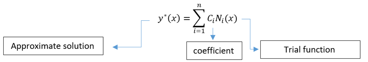
This approximate solution is substituted into the differential equation. In differential equation mode, we can write:
![]()
And an equation for the error, called the residual, is an error function, and we can write it like this:
![]()
If the value of y*(x) is an exact value, the error function is equal to zero.
If we multiply each trial function by the residual and set the integral of this product to zero, we can calculate the unknown coefficients that minimize the residual. This gives us an approximate solution to the differential equation. Now, any unknown coefficient can be calculated using the error function:
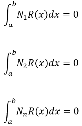
Each element must have its own displacement function. This is a more widely applicable approach than the principle of minimum potential energy. To solve the singularity problem, we must use boundary conditions. We need boundary condition to keep the structure in place rather than moving as a rigid body, so “a” and “b” is the boundary condition of our problem.
You’re bored, right?! Let’s solve an example to understand it better.
3.4.4. Derivation of the Stiffness Matrix for a Spring element
We will now derive the stiffness matrix for a one-dimensional linear spring using the direct equilibrium approach. This spring obeys Hooke’s law and resists forces only in the direction of the spring.
We now want to develop a relationship between nodal forces and nodal displacements for a spring element. The stiffness matrix will be based on this relationship. As a result, we propose the following relationship between the nodal force matrix and the nodal displacement matrix:
Consider the linear spring element subjected to the resulting nodal tensile forces T directed along the spring axial direction x, as shown in Figur3, to be in equilibrium.
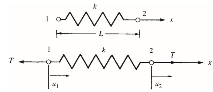
Figure 4: Spring subjected to tensile forces and in the equilibrium state
The Strain/Displacement and Stress/Strain Relationships must be defined. The difference in nodal displacements represents the total deformation of the spring as follows:
![]()
Instead of the stress/strain relationship, consider the force/deformation relationship:
![]()
Now we can write:
![]()
We can rewrite the equation by substituting the force components as follows:
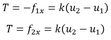
Now expressing the equations above in a single matrix equation:
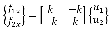
Then, for structures composed of more than one element
t, we must assemble the element equations to obtain the global equations and introduce boundary conditions.
![]()
where ![]() and
and ![]() are now element stiffness and force matrices expressed in a global reference frame.
are now element stiffness and force matrices expressed in a global reference frame.
The displacements are then calculated by imposing boundary conditions, such as support conditions, and simultaneously solving a system of equations as:
![]()
Finally, the element forces are determined by back-substitution.
3.5. Step 5: Assemble the Element Equations to get the Global or Total Equations, and then add Boundary Conditions
After deriving the stiffness matrix for each individual element, we now need to combine them to model the entire structure.
This process is called assembly.
In Step 5, we assemble all the element nodal equilibrium equations into a complete set of global nodal equilibrium equations.
In simple terms, we piece together all the small elements to form the big puzzle of the structure.
There are two main approaches for assembling the global system:
-
Standard Assembly Method:
Systematically add the contributions of each element into the global stiffness matrix based on shared nodes. -
Direct Stiffness Method:
A more direct and often simpler method based on applying nodal force equilibrium directly.
In this method, we assume the equilibrium of forces at each node from the start, ensuring all elements fit together seamlessly.
🔵 Important Concept:
The continuity or compatibility of the structure is crucial during assembly.
This means that:
-
The structure must stay together (no tears or separations between elements).
-
The displacements at shared nodes between elements must be consistent.
Finally, boundary conditions (such as fixed supports, rollers, or prescribed displacements) are applied to the global system.
These conditions are necessary to make the system solvable and physically meaningful.
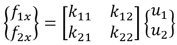
The final assembled or global equation in matrix form is as follows:
![]()
As we said before, {F} is the vector of global nodal forces, [K] is the structure global or total stiffness matrix (for most problems, the global stiffness matrix is square and symmetric), and {u} is the vector of known and unknown nodal degrees of freedom or generalized displacements of the structure.
The element stiffness matrix defines how much each node in the element will displace when a set of forces and moments is applied to the nodes. Moreover, it is the key to solving the displacements at every node. Figure 5 shows just one element, but our overall mesh will be made up of many more elements.
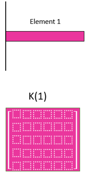
Figure 5: Stiffness matrix for one element
For example, in a 2D beam, we can assemble the individual stiffness matrices of all the elements (figure 6) into a huge global stiffness matrix that defines how the entire structure will displace when loads are applied to it.
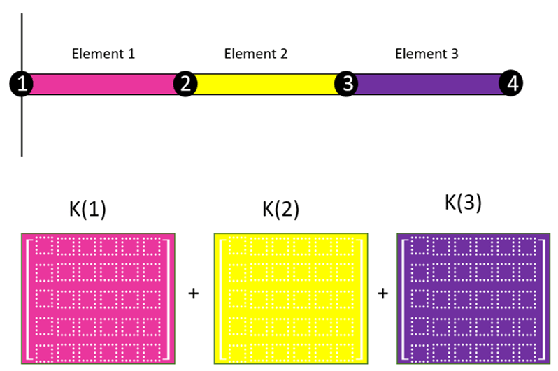
Figure 6: Stiffness matrices for each element of the 2D beam
Like the element stiffness matrix, the global stiffness matrix is a square matrix, and the number of rows and columns is equal to the total number of degrees of freedom in the model. The element stiffness matrices are assembled together to form the global stiffness matrix based on how the elements are connected together. Figure 7 shows that elements 1 and 2 are connected at node 2, and it tells us that since these two elements are connected at the same node, the displacement for both elements must be the same at the common node.
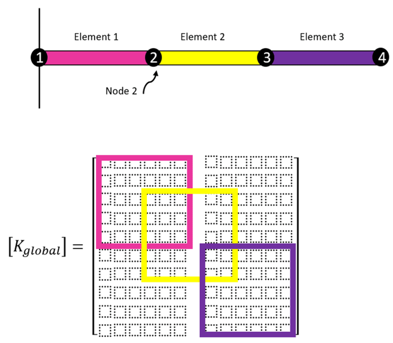
Figure 7: Global stiffness matrix of a 2D beam element
So when we assemble the global stiffness matrix, the terms in the element stiffness matrices corresponding to node 2 should be summed for each degree of freedom. Figure 7 shows that element 3 is not connected to node 2, so this element’s stiffness matrix should not affect the displacements at node 2. Figure 7 shows the actual global stiffness matrix for this model.
🔹 Key takeaway:
In Step 5, we build the global picture by connecting all the elements and ensuring the structure acts as a single, continuous body.
Note: You can learn more about mesh and meshing in Abaqus just by reading this article “The Best Guide to Abaqus Mesh“.
3.6. Step 6: Determine the Unknown Degrees of Freedom
Now that we have assembled the global system of equations and applied boundary conditions, it’s time to solve for the unknown nodal displacements.
The global equilibrium equations take the form:
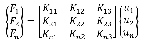
The total number of unknowns (n) corresponds to the total number of free nodal degrees of freedom in the structure.
After incorporating boundary conditions (such as fixed displacements or prescribed forces), the system becomes solvable.
We can use different numerical methods to solve the resulting set of simultaneous algebraic equations:
-
Direct Methods:
Techniques like Gauss elimination systematically reduce the system to find an exact solution. -
Iterative Methods:
Approaches like Gauss-Seidel or Conjugate Gradient are useful, especially for very large systems where direct methods become computationally expensive.
🔹 Key takeaway:
In Step 6, we compute the primary unknowns — the nodal displacements — by solving the system of equations.
3.7. Step 7: Solution for the Element Strains and Stresses
After solving for the unknown nodal displacements, we can now calculate important secondary quantities — namely, strain and stress within each element.
This is possible because strain and stress are directly related to displacement:
-
Using the displacement field, we compute the strain within each element (using strain-displacement relations like ε = du/dx for 1D problems).
-
Then, using the material’s stress-strain relationship (such as Hooke’s Law), we compute the stress.
In structural stress analysis problems, we are often particularly interested in:
-
Strains — how much the material deforms locally.
-
Stresses — how much internal force is acting within the material.
-
Moments and shear forces — especially for beam or frame structures.
🔹 Key takeaway:
In Step 7, we translate the computed displacements into real-world quantities (strain, stress, moment, shear) that engineers use to assess the safety and performance of structures.
3.8. Step 8: Analyze the Result of finite element analysis
The final step in the finite element method process is analyzing and interpreting the results to make informed engineering decisions.
The computed displacements, strains, stresses, and other quantities must be carefully evaluated to:
-
Identify critical regions with high stresses or large deformations.
-
Check if the structure meets design criteria for strength, stiffness, and safety.
-
Optimize the design by making modifications where necessary.
To assist in this process, post-processing software (like visualization tools in Abaqus, Ansys, or other FEA programs) presents the results graphically:
-
Color contour plots for stress and displacement.
-
Deformed shape views.
-
Animation of load applications.
-
Extracted numerical data for detailed studies.
🔹 Key takeaway:
Step 8 is where engineering judgment is vital: understanding what the results mean for your real-world structure or product.
🎬 Bonus for you:
Since you’ve followed along with this beginner-friendly guide, there’s a special video waiting for you!
It shows the finite element method in action using Abaqus, connecting all the steps you’ve learned here.
4. What’s the Difference Between FEM and FEA (Finite Element Analysis)?
By now, you’ve seen that the Finite Element Method (FEM) is an incredibly powerful tool for solving complex engineering problems.
But a common question pops up among beginners:
Are FEM and FEA the same thing? If not, what’s the difference?
Let’s break it down.
🔹 FEM: The Theory Behind It All
Finite Element Method (FEM) refers to the mathematical and theoretical framework used to break down complex problems into smaller, solvable parts.
It includes:
-
Mathematical approaches like the Galerkin method, weighted residual method, and numerical integration methods.
-
The development of element equations, stiffness matrices, and system assemblies.
You can think of FEM as the “science textbook” full of equations, principles, and derivations that define how things should behave when applying finite element techniques.
🔹 FEA: The Practical Application
Finite Element Analysis (FEA), on the other hand, refers to the practical use of FEM to solve real-world engineering problems — often with the help of software.
When you hear engineers talk about running an “FEA simulation” or using “FEA software,” they are applying the theory of FEM to analyze physical behavior, like:
-
Heat transfer
-
Structural strength
-
Vibrations
-
Fluid flow
-
Buckling, fatigue, and more
In short:
FEM = The method and theory
FEA = The real-world application (usually with the help of computer software)
🔥 Why Has FEA Become So Popular?
Several reasons explain the explosion of FEA usage in industries:
-
User-Friendly Software:
In the past, using FEM required deep mathematical knowledge. Today, software hides the complicated math behind simple, intuitive interfaces.
(You mostly see CAD models and colorful contour plots instead of scary equations!) -
Cost-Effective Design Optimization:
FEA provides a cheaper, faster way to optimize products without building expensive prototypes or performing endless physical tests. -
Increasing Problem Complexity:
Modern engineering problems (think space rockets, biomedical implants, electric vehicles) are so complex that closed-form (exact) solutions are impossible.
FEA offers an efficient way to get approximate but reliable answers. -
Changing Work Habits:
Some engineers now rely heavily on FEA software, letting it handle heavy mathematical lifting rather than solving problems manually.
What’s Next After FEA?
While FEA is dominant today, new techniques like Meshless Methods are emerging.
As designs become more organic (think aerodynamic car bodies or biomechanical prosthetics), meshing becomes harder and more time-consuming.
Meshless methods promise to solve problems without needing traditional meshing, offering new opportunities for the future of computational engineering.
So while FEA is incredibly powerful today, always keep an eye on where the technology is heading!
What is included in this package?
Video
5 Workshops
Theory &
Practice
Files
5. A Simple Real-World Example of FEM
After you have a cup of coffee, to make everything more concrete, let’s go through a very simple example of how the Finite Element Method is applied to a real-world problem.
The modern form of the finite element method can routinely solve many industrial problems. They enable fundamental understanding and allow predictive analysis for product design. We want to simulate an I-shaped beam under the constricted transfer loading P.
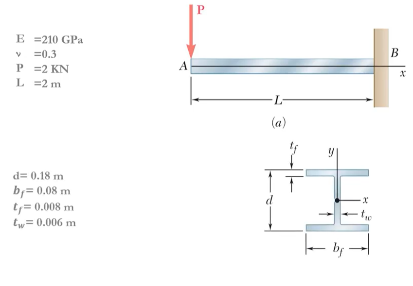
Figure 8: Description of the problem (for FEA analysis)
In the remaining part of this post, I have explained the finite element analysis steps. If you are interested in FEA analysis learning or you are a student who needs to start finite element analysis for your project, I recommend checking the Abaqus tutorial page.
5.1. Step 1: Modeling
At first, we can model it in ABAQUS as a static model with the Part module. An ABAQUS/CAE model is built using parts as its foundation. Each part is created using the Part module, and instances of the parts are assembled using the Assembly module.
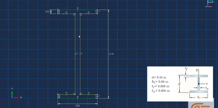
Figure 9: Creating the model in the Part module
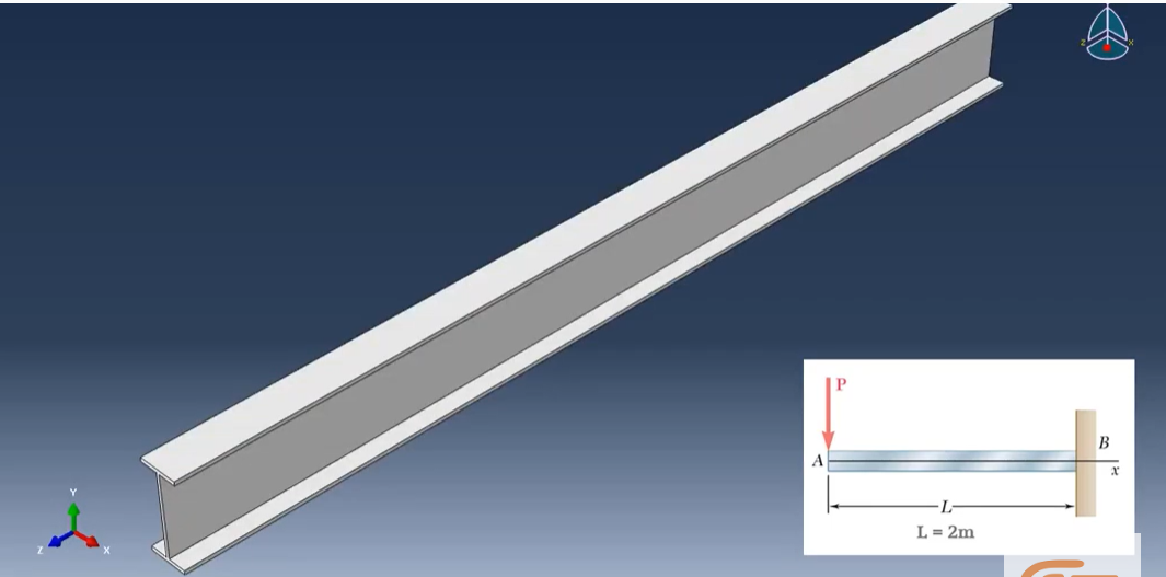
Figure 10: Created model in 3D shape
5.2. Step 2: Choose the material of the structure
The mechanical property of your material can be entered in ABAQUS using the Property module. By specifying them at a variety of temperatures, material properties become temperature-dependent. A material property can sometimes be defined as a function of ABAQUS-calculated variables; For instance, stress must be given as a function of equivalent plastic strain to define a work-hardening curve.
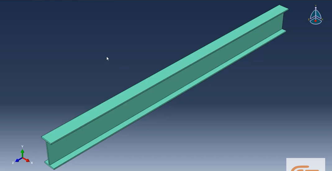
Figure 11: Assigned material properties on the model
5.3. Step 3: Assemble the structure
At the Assembly module, we can select any structure component to assemble. Using an organizational scheme that is analogous to the physical assembly, analysts can create a finite element mesh with the help of ABAQUS’s assembly interface. Part instances are the assemblies of individual components in ABAQUS.
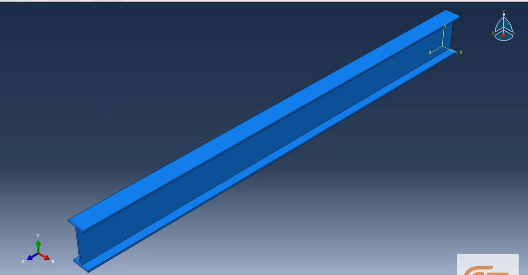
Figure 12: model instance in the Assembly module
5.4. Step 4: Choose the solution method
In the Step module, we want to define the problem-solving approach. To solve this example, we can choose “Static, general.” Abaqus is based on the idea of breaking up the problem history into steps. An Abaqus step is any convenient loading history phase, such as a static, dynamic, or thermal transient. In its simplest form, a step can be nothing more than a static analysis of how a load changes from one magnitude to another.
5.5. Step 5: Create boundary condition
We can use the Load module in ABAQUS to create boundary conditions and insert loading. The model’s boundary conditions and loading conditions can be defined and managed with the help of the Load module.
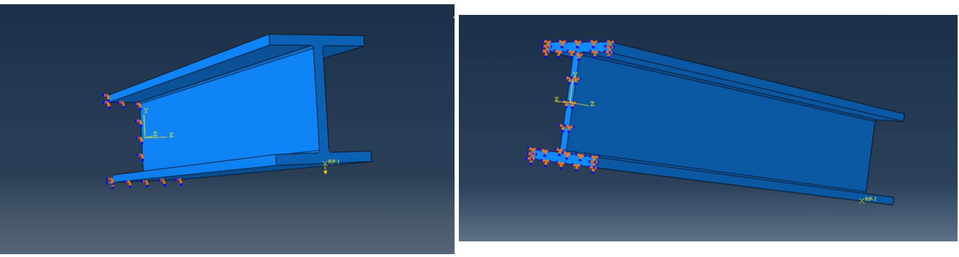
Figure 13: Loading and boundary conditions
5.6. Step 6: Choose the element type
We should select the element type when meshing the model to achieve a satisfactory and sensible solution to the problem. An FEA model defines a mesh, which is an arrangement of finite elements. A mesh can be defined on a part or an assembly in Abaqus/CAE. The process of discretizing geometry into a finite element representation mesh is known as meshing.
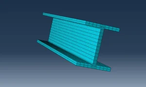
Figure 14: Meshed part
5.7. Step 7: result
In the Visualization module, you can select the results you want to display. For example, you can select stress or strain and see the results in all elements of the model. In this module, you can plot the results of any variable you want. FEA analysis results are the outcome of the FEA analysis process, and engineers use these results for their next calculations.
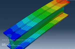
Figure 15: Results in the Visualization module in Abaqus (the outcome of FEA analysis)
You can find more examples, Free pdfs, free tutorial video packages and more in Abaqus Examples article.
What is FEM simulation?
A FEM simulation shows how a component or material reacts to certain influences. It is based on the finite element method (FEM). With this numerical calculation method, a component or an entire assembly is divided into a finite number of elements (sub-areas).
6. Application of FEM (finite element analysis)
Now we come to the exciting part of the story. Before we start, close your eyes and relax for 10 seconds!
“Where is FEM used, and why is it such a big deal?”
Let’s find out!
Both structural and nonstructural issues can be examined using the finite element method.
The most typical structural areas are:
- Stress analysis: From trusses to frames, FEM helps determine where stresses and strains occur in structures.
- Buckling, such as in columns, frames, and vessels: In critical components like columns and vessels, FEM can predict potential failures due to buckling.
- Vibration analysis, such as in vibratory equipment: Whether it’s machinery or buildings, FEM aids in understanding and mitigating vibrations that could lead to failure.
- Impact problems, including crash analysis of vehicles: FEM is widely used in the automotive industry to simulate crashes, ensuring safety features are designed to withstand impact.
And nonstructural problems include:
- Heat transfer, such as in electronic devices emitting heat as in a personal computer microprocessor chip
- Fluid flow, including seepage through porous media: Simulating fluid dynamics, such as seepage through porous materials, is made simple with FEM.
- Distribution of electric or magnetic potential: FEM is instrumental in predicting how electric and magnetic fields interact in complex systems.
- Biomechanics: Analyzing the Human Body with FEM
Did you know that the human body itself is an intricate composite material? With FEM, you can model the human spine, skull, joints, and even dental implants. Understanding the stress distribution in these areas has revolutionized medical engineering, from creating stronger implants to better understanding human biomechanics.
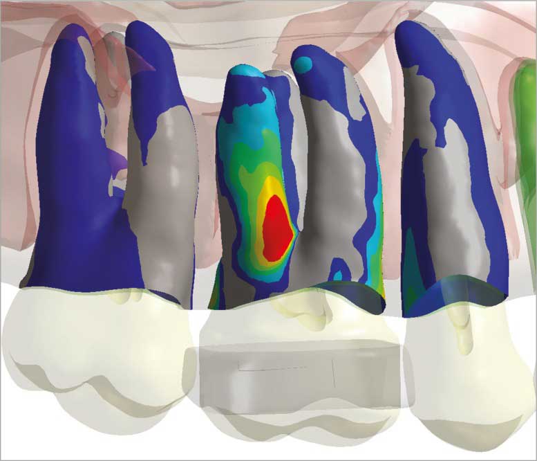
Areas of stress concentration [Ref]
IF you are interested in biomechanical structures and want to see some practical examples in Abaqus, I think this package can help you a lot:
Bio-Mechanical Abaqus simulation Full package
Now, we’ll talk about some common uses for the finite element method or engineering FEA. These applications will demonstrate the variety, size, and complexity of the problems that can be solved using the FEM method, as well as the typical discretization process and types of elements used. For example, 120 nodes and 297 plane strain triangular elements were used to model the hydraulic cylinder rod end in figure 16. In addition, symmetry was applied to the entire rod end so that only half of it needed to be analyzed, as depicted. This analysis aimed to find places in the rod end where there was a lot of stress. This is a simple kind of finite element analysis (FEA analysis) in industrial applications.
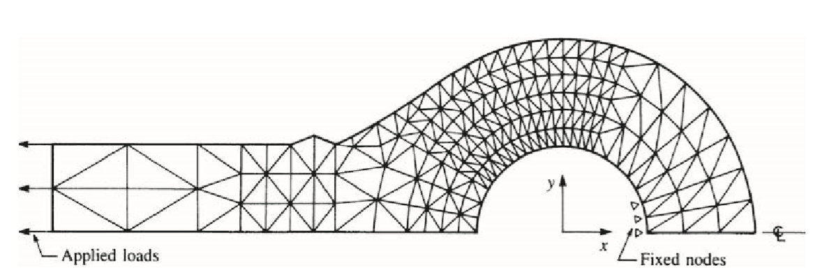
Figure 16: Two-dimensional analysis of a hydraulic cylinder rod end (120 nodes, 297 plane strain triangular elements)
6.1. Aerospace & FEA analysis
In industries like aerospace and automotive, composite materials have become essential due to their high strength-to-weight ratio. However, these materials come with challenges, including high costs and complex behaviors. FEM is essential for simulating composite materials under extreme conditions, helping to optimize designs and performance.
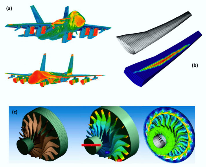
Some of FEM applications in Aerospace[Ref]
6.2. Naval & FEA analysis
In the naval industry, FEM is used extensively to predict the mechanical properties of materials used in ships and submarines. It helps optimize designs for reduced weight, enhanced durability, and improved structural integrity, ensuring vessels perform under extreme conditions while maximizing efficiency.
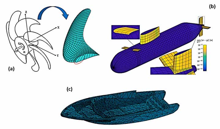
Some of FEM applications in Naval[Ref]
6.3. Sports & FEA analysis
The sports industry has embraced composite materials, particularly in high-performance sports equipment, like racing bicycles or golf clubs. By using FEM, engineers can design lighter, stronger, and more durable materials that improve athletes’ performance, pushing the boundaries of what’s possible.
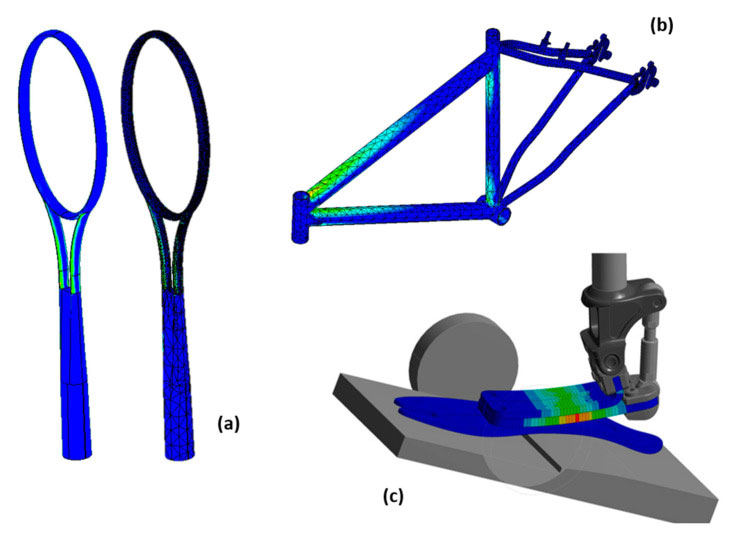
Some of FEM applications in Sports equipment[Ref]
7. Strengths and Limitations of the Finite Element Method (FEM)
Like any powerful tool, the Finite Element Method (FEM) has its strengths and weaknesses. Let’s explore what makes FEM so popular — and where its challenges lie.
✅ Strengths of FEM
FEM offers several key advantages compared to traditional methods of solving engineering problems:
-
Easily Handles Complex Geometries:
Designing and analyzing bodies with irregular, intricate shapes is simple with FEM. -
Versatile Material Modeling:
FEM can model structures made from multiple materials or materials with varying properties (even within a single element). -
Flexible Boundary Conditions:
It manages an infinite variety of boundary conditions, including fixed supports, pressures, thermal loads, and more. -
Localized Refinement:
Engineers can refine the mesh where needed, using smaller elements in critical regions for higher accuracy without overloading the entire model. -
Nonlinear Problem Solving:
FEM can simulate nonlinear material behavior (like plastic deformation) and large deformations, which traditional methods struggle with. -
Wide Range of Applications:
It supports simulations in structural mechanics, heat transfer, fluid flow, electromagnetics, and beyond. -
User-Friendly and Supported:
Modern software tools (like ANSYS, Abaqus, COMSOL, and even SolidWorks) make FEM accessible, with many tutorials, books, and resources available. -
Results-Focused:
Engineers can quickly generate results like stress, displacement, thermal gradients, and pressure fields — without diving deep into hand calculations.
⚠️ Limitations of FEM
Despite its power, FEM does come with some important limitations:
-
High Computational Cost:
A fine mesh dramatically increases the number of elements and nodes, which demands more memory, processing power, and solution time. -
Approximate Solutions Only:
FEM provides numerical approximations — not exact answers.
Errors are minimized across the whole domain, but true accuracy is guaranteed only at specific points (usually the nodes). -
Idealization of Reality:
Simplifying real-world structures into idealized models can introduce inaccuracies, especially for highly complex or organic shapes. -
Mesh Dependency:
Poorly created meshes can cause incorrect or unstable results.
Good meshing often requires experience and judgment. -
Software Dependency:
Although FEM software is easier to use today, a deep understanding of the underlying physics and numerical methods is still critical to get meaningful results.
Quick Summary Table
| Strengths | Limitations |
|---|---|
| Solves complex geometries | Requires significant computational resources |
| Models varied materials easily | Only approximate solutions |
| Handles complex boundary conditions | Accuracy depends heavily on mesh quality |
| Simulates nonlinear behavior | Idealization of real-world objects is not perfect |
| User-friendly tools and abundant resources | Risk of misuse without theoretical understanding |
8. FEM Software
Before purchasing any software, a user interested in supporting finite element programs and designing finite element model should carefully consult the vendor. However, to give you an idea of the various commercial, and personal computer programs currently available for problem-solving using the finite element method, we provide a partial list of the currently available programs.
- Autodesk Simulation Multiphysics
- Abaqus
- ANSYS
- COSMOS/M
- GT-STRUDL
- LS-DYNA
- MARC
- MSC/NASTRAN
- NISA
- Pro/MECHANICA
- SAP2000
- STARDYNE
What Is the Place of FEA among Other Tools of Computer-Aided Engineering?
FEA is one of many computer-aided engineering (CAE) tools used in the mechanical design process. Other CAE tools include fluid analysis and mechanical analysis, commonly referred to as computational fluid dynamics (CFD). These three major CAE tools, FEA, CFD, and motion analysis, are integrated into Computer Aided Design (CAD), which is the hub of all his CAE applications. Geometry, material properties, and certain boundary conditions can be exchanged between CAD and add-ins and among add-ins themselves. FEA, CFD, and mechanistic analysis were developed independently and are based on different numerical methods. CAE tools are standalone programs and are not add-ins to CAD, but they can be connected to CAD.
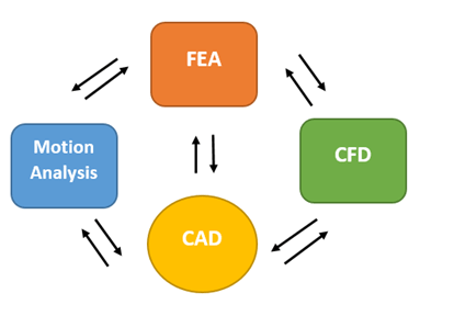
Figure – CAE applications such as FEA, CFD, and Motion Analysis are add-ins to CAD,They can exchange data with CAD and among themselves
8.1 Verification and Validation of FEA Results
Verification and validation as applied to design analysis with FEA are defined as follows:
- Verification checks whether the mathematical model has been discretized and solved correctly.
- Validation determines if the solution correctly represents the reality from the perspective of the intended use of the results. It checks if the results correctly describe the real-life behavior of the analyzed system.
It checks whether the results accurately describe the actual behavior of the system under analysis.
A model with mesh errors will fail the verification test. For example, using elements that are too large will result in an incorrect solution. The check fails if discretization errors or solution errors invalidate the results. Convergent analysis will uncover issues that cause testing to fail.
A model with an incorrect load definition will fail the verification test because verification is only concerned with the correctness of the mathematical model solution and not whether the mathematical model itself is correct. Establishing the correctness of a mathematical model as well as the correctness of its solution is the process of validation. Validation will fail if there is a conceptual error in the definition of the mathematical model. Concept errors are much more dangerous than discrete errors.
They can escape the attention of the modeler, especially because there is no clearly defined process for detecting conceptual errors. The only protection against validation errors is a precise definition of the problem being analyzed. Verification checks the numerical solution of a mathematical model. Validation checks how well the results apply to reality. The flowchart also shows errors introduced at each step of the FEA project.
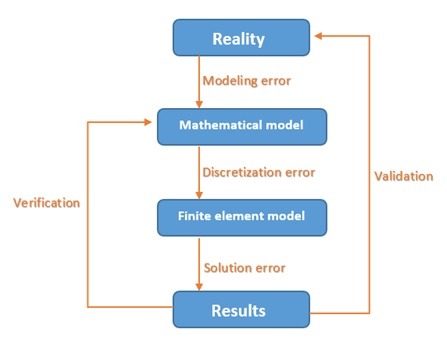
Figure – Verification and validation of FEA results and the errors introduced at each step of the FEA project
9. Understanding the Common Causes of Errors in Finite Element Analysis (FEA)
Finite Element Analysis (FEA) has revolutionized the way engineers and designers approach complex simulations, helping them solve problems across diverse fields from aerospace to biomechanics. However, like any powerful tool, FEA isn’t immune to errors. A single misstep can lead to inaccurate results, which could have significant real-world consequences. Understanding where these errors stem from is essential for improving the reliability of your simulations.
In this post, we’ll explore the key sources of error in Finite Element Analysis and how you can avoid them.
- Mesh Quality: The Foundation of Accuracy
One of the most critical aspects of FEA is the mesh—the discretization of the model into smaller, simpler elements. The quality and density of the mesh play a massive role in the accuracy of the results.
- Boundary Conditions: Setting the Stage
Accurate boundary conditions are crucial for the FEA to reflect real-world behavior. Errors in boundary conditions can lead to wildly incorrect results.
- Material Properties: The Heart of the Model
The accuracy of your FEA results is heavily dependent on the material properties you input. Incorrect material data can lead to vast errors in simulation outcomes.
- Solver Convergence Issues: When the Solution Won’t Settle
Solver convergence is a common issue in FEA that often arises when the problem is too complex for the chosen settings. Convergence refers to the process where the numerical solution stabilizes after several iterations.
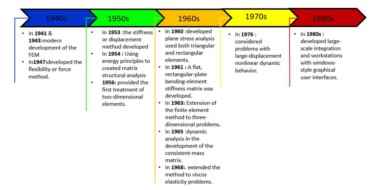
10. A Brief Introduction to Finite Element Analysis History
Now, let’s make an introduction to finite element analysis history and see where it come from.
- 1941 & 1943, With the work of Hrennikoff and McHenry in the field of structural engineering, the modern development of the finite element method started in the 1940s.
- In 1947, Levy developed the flexibility or force method, and his study recommended that a different approach should be used in 1953.
- In 1954, Using energy principles, Argyris and Kelsey created matrix structural analysis techniques.
- In 1956 Turner et al. provided the first treatment of two-dimensional elements. They created stiffness matrices for two-dimensional triangular and rectangular elements, beam elements, and truss elements in plane stress.
- In 1960 Clough developed the term “finite element” when plane stress analysis used both triangular and rectangular elements.
- In 1961, A flat, rectangular-plate bending-element stiffness matrix was developed by Melosh.
- In 1963 Extension of the finite element method to three-dimensional problems with the development of a tetrahedral stiffness matrix was done by Melosh.
- In 1963 Melosh’s realization that the finite element method could be set up in terms of a variational formulation, it began to be used to solve nonstructural applications.
- In 1965 Archer considered dynamic analysis in the development of the consistent-mass matrix.
- In 1968, Zienkiewicz et al. extended the method to visco elasticity problems. (Introduction to finite element method)
- In 1969, using weighted residual techniques, first by Szabo and Lee to obtain the elasticity equations previously employed in structural analysis.
- In 1976, Belytschko considered problems associated with large-displacement nonlinear dynamic behavior and improved numerical techniques for solving the resulting systems of equations.
- In the late 1970s and early 1980s, Large-scale integration and workstations with windows-style graphical user interfaces were first developed, along with the computer mouse.
11. Conclusion
In this post, we explored the basics of the Finite Element Method (FEM) — from what it is, to how it works, to where it’s used.
You now know that FEM is not just a mathematical tool, but a game-changer that engineers use every day to design safer bridges, stronger aircraft, faster cars, and even life-saving medical devices.
Sure, it has its complexities.
Yes, it has limitations.
But FEM allows us to tackle problems that traditional hand calculations simply can’t handle — and that’s why it’s so essential in modern engineering.
As an engineering student, learning FEM gives you a huge advantage.
It’s a skill highly valued in industries like automotive, aerospace, biomedical, energy, civil engineering, and more.
Whether you aim to design rockets, skyscrapers, prosthetic limbs, or the next electric vehicle — FEM is part of your toolkit for innovation.
I am looking for a complete and detailed FEM. According to this article, it sounds like the one I need. thanks