
Abaqus Mesh, Top-down mesh, Bottom-up mesh, and Abaqus structured mesh are the common words you hear when it comes to meshing in Abaqus. The differences? The Exact differences? Which one should I use? Maybe no one knows the exact answers. What about the techniques we can use in Abaqus?
One of the key aspects of Finite Element Method (FEM) is the concept of meshing. It involves dividing a complex domain into smaller, simpler elements. These elements are then connected together to form a mesh, which serves as the basis for solving the governing equations of the problem.
In this article, besides the meshing basics you must know to generate efficient mesh on your model, we discuss the Abaqus Mesh module capabilities and the Abaqus meshing techniques you can use. This article tries to give you a better insight into the meshing process when you use Abaqus for your FEM analyses.
1. What is the mesh in Abaqus? | Abaqus Mesh
Inaccurate meshing can lead to errors in the results, which can prove to be costly in terms of time, effort, and resources. In contrast, proper meshing techniques can significantly improve the accuracy of the results and reduce the risk of errors. With this intro let’s start our discussion by Abaqus mesh definition.

Master meshing in Abaqus! This tutorial dives deep into meshing techniques, guiding you from basic concepts to advanced tools. Learn how to create accurate and reliable meshes for your finite element analysis, ultimately taking your Abaqus skills to the next level:
1.1. Mesh definition in FEM
In FEM, mesh refers to the division of a continuous domain into smaller, finite subdomains known as elements. These elements are geometrically simple and connected to each other through nodes or vertices. The process of dividing the domain into elements is known as meshing, and it plays a crucial role in the accuracy and efficiency of FEM.
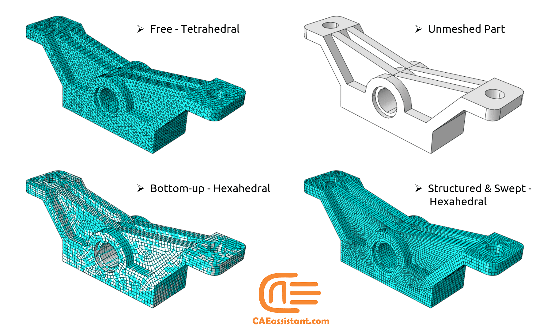
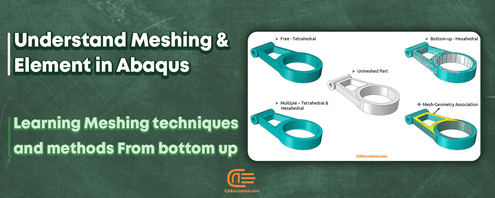
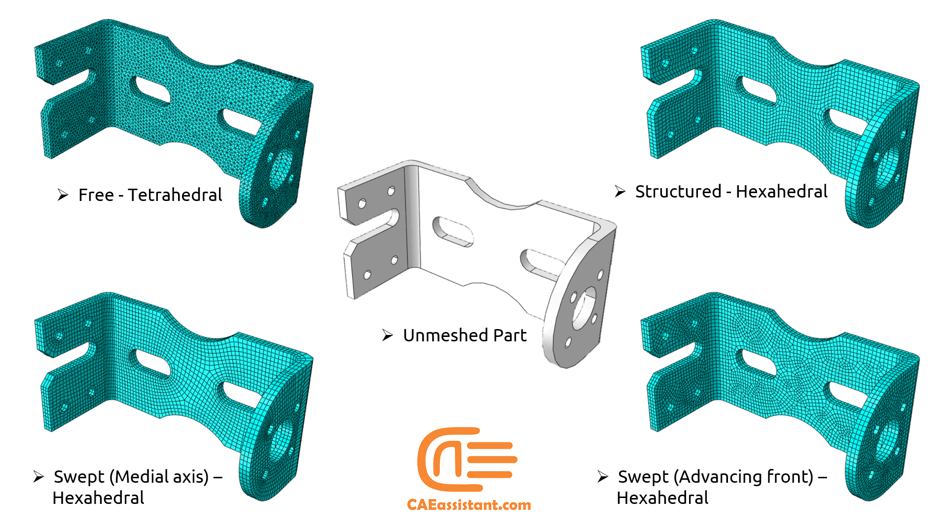
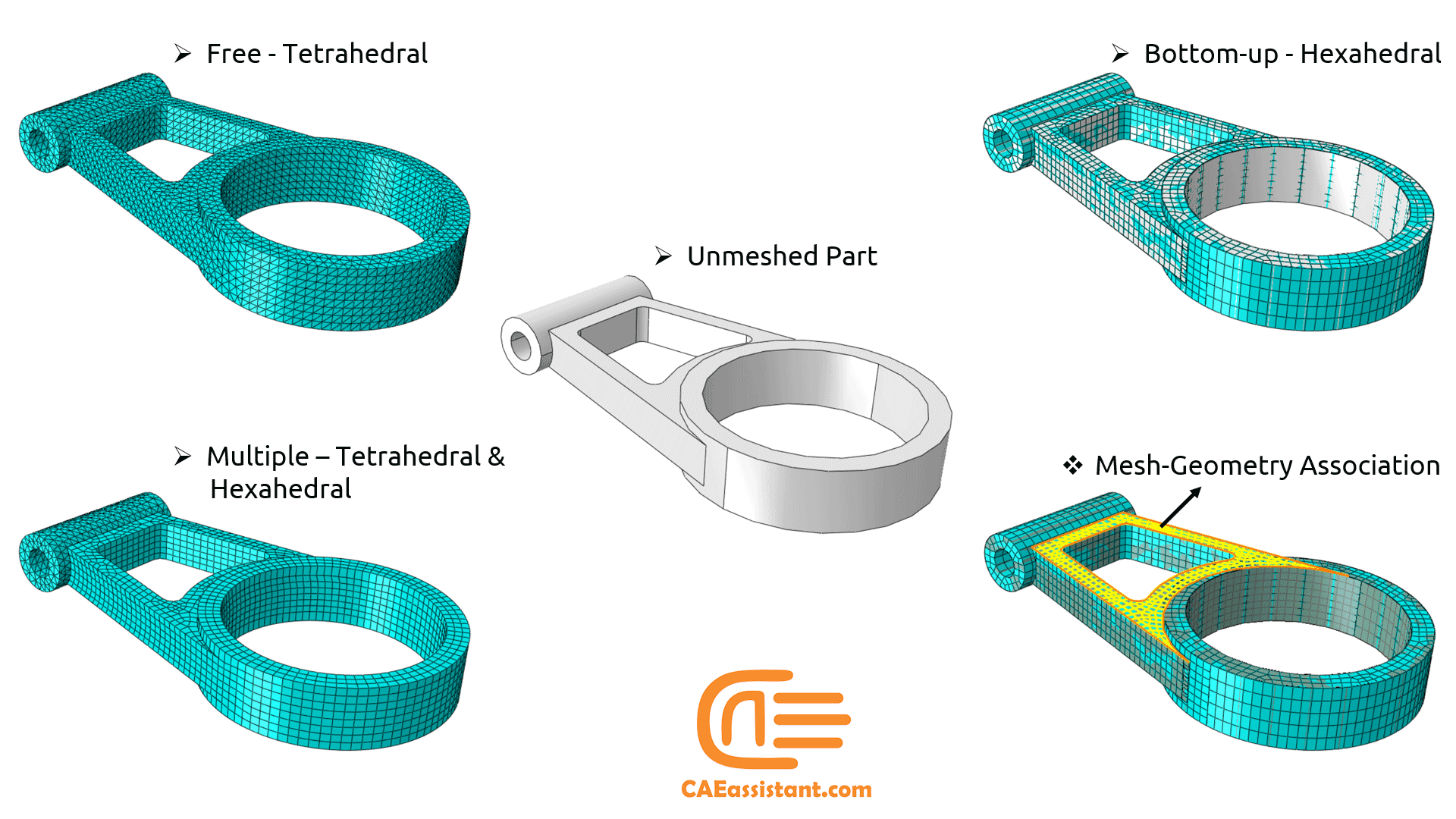
This picture shows you how you can mesh a part with different techniques and methods in Abaqus. But the golden question is, which one should I use for my simulation?? That is a very good question, right? How about something more simple; how to use these techniques to get such a clean meshing? Learn with this example and more in “Different Techniques for Meshing in Abaqus” tutorial.
1.3. Mesh Convergence | Mesh sensitivity analysis Abaqus
It is important that you use a sufficiently refined mesh to ensure that the results from your Abaqus simulation are acceptable (Mesh sensitivity analysis Abaqus) because:
- The solution of FEA is highly dependent on mesh size and the type of elements.
- Coarse meshes can yield inaccurate results; While computer resources required to run your simulation also increase as the mesh is refined.
Typically, the numerical solution provided by your model will tend toward a unique value as you increase the mesh density. The mesh is said to be “Converged” when further mesh refinement produces a negligible change in the solution
The connecting lug shown in figure 1 is analyzed using four different mesh densities as an example of a mesh convergence study. The coarse mesh based on Table 1 predicts inaccurate displacements at the bottom of the hole, but the normal, fine, and very fine meshes all predict similar results. The normal mesh is, therefore, converged as far as the displacements are concerned.
1.2. Impact of Mesh on simulation results
One of the primary roles of meshing in Abaqus software is to ensure that the user-defined boundary conditions are applied correctly. These boundary conditions determine the behavior of the physical system under the given constraints. And any errors in their application can lead to an incorrect analysis. A well-meshed model ensures that the boundary conditions are appropriately represented in the simulation, leading to reliable results.
Meshing also plays a critical role in dealing with complex geometries. It is often challenging to model real-world structures accurately due to their intricate and irregular shapes. By dividing the domain into smaller elements, meshing helps to approximate these complex geometries. This allows for a more accurate representation of the physical system.
Another significant aspect of meshing in Abaqus software is its effect on computation time. A well-meshed model not only improves the accuracy of the results but also reduces the computation time. This is because elements with an appropriate size and shape can better represent the behavior of the physical system, thereby reducing the number of elements and nodes required for the simulation. As a result, the simulation time is reduced, making the overall analysis more efficient.
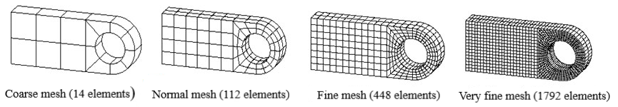
Figure 1: Different mesh sizes on the connecting lug
Table 1: Simulation results for different mesh sizes
| Mesh | Displacement of bottom of hole | Stress at bottom of hole | Relative CPU time |
| Coarse | 2.01E–4 | 180.E6 | 0.26 |
| Normal | 3.13E–4 | 311.E6 | 1.0 |
| Fine | 3.14E–4 | 332.E6 | 2.7 |
| Very fine | 3.15E–4 | 345.E6 | 22.5 |
2. Abaqus Mesh module
The Mesh module contains tools that allow you to generate meshes on parts and assemblies created within Abaqus/CAE. In addition, the Abaqus Mesh module contains functions that verify an existing mesh.
2.1. Abaqus mesh module features
The Abaqus Mesh module provides the following features:
- Prescribing mesh density: The Mesh module provides tools for prescribing mesh density at local and global levels.
- Model coloring indicator: This feature indicates the meshing technique assigned to each region in the model.
- Variety of mesh controls: Mesh module provides a variety of options to control the mesh you generated for the model such as:
- Element shape
- Meshing technique
- Meshing algorithm
- Adaptive remeshing rule
- Assigning element types: A tool for assigning Abaqus/Standard and Abaqus/Explicit element types to mesh elements.
- Verify mesh quality: Abaqus provides a set of tools in the Mesh module that allow you to verify the quality of your mesh and obtain information about the nodes and elements in the mesh.
- Refining and improving the mesh: Abaqus provides some tools to refine and improve the mesh quality everywhere needed.
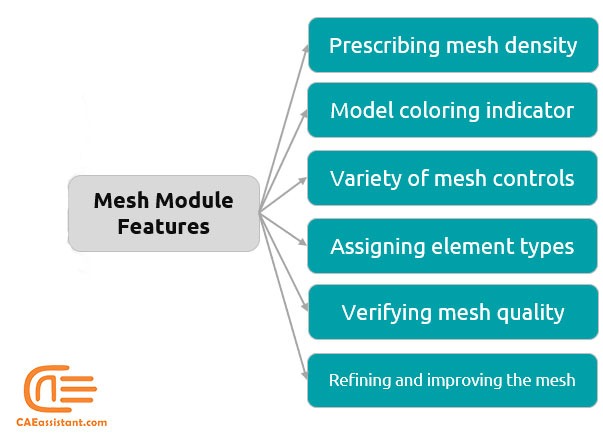
Figure 2: Mesh module features in Abaqus
2.2. Abaqus mesh module toolbox
You can access all the Mesh module tools through either the main menu bar or the toolbox. Here are all the tools in the Mesh module toolbox including hidden icons.

Figure 3: Mesh module toolbox in Abaqus
2.3. Abaqus meshing color coding
When the Mesh defaults color mapping is selected, Abaqus/CAE uses different colors to indicate which meshing technique, if any, is currently assigned to a region.
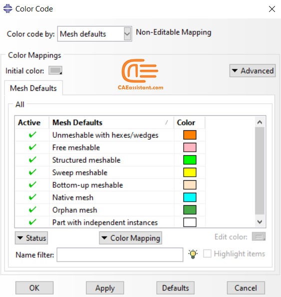
Figure 4: Mesh module color coding
Here is the list of colors in figure 4:
- Orange: Unmeshable with hexes/wedges
- Rose: Free meshable
- Light Green: Structured meshable
- Yellow: Sweep meshable
- Light Orange: Bottom-up meshable
- Aqua: Native mesh
- Green: Orphan mesh
- White: Part with independent instances
3. Abaqus Mesh terminology
This section provides brief explanations of terms and concepts that you must understand to use the Mesh module effectively. It gives you an overview of the functions available and describes the role that each function plays in the mesh creation process.
3.1. Meshing Process
To create an acceptable mesh, you use the following process:
- Assign mesh attributes and set mesh controls
The Mesh module provides a variety of tools that allow you to specify different mesh characteristics, such as mesh density, element shape, and element type.
- Generate the mesh
The Mesh module uses a variety of techniques to generate meshes. The different mesh techniques provide you with different levels of control over the mesh.
- Refine the mesh
The Mesh module provides a variety of tools that allow you to refine the mesh:
The seeding tools allow you to adjust the mesh density in selected regions.
The Partition toolset allows you to partition complex models into simpler subregions.
The Virtual Topology toolset allows you to simplify your model by combining small faces and edges with adjacent faces and edges.
The Edit Mesh toolset allows you to make minor adjustments to your mesh.
- Optimize the mesh
You can assign remeshing rules to regions of your model. Remeshing rules enable successive refinement of your mesh where each refinement is based on the results of an analysis.
- Verify the mesh
The verification tools provide you with information concerning the quality of the elements used in a mesh.
The meshing process steps are shown in the figure 5.
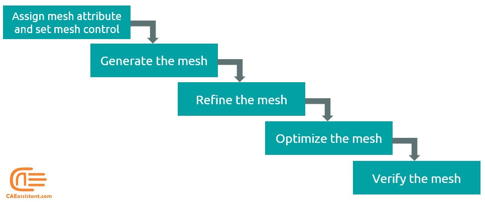
Figure 5: Meshing process steps in Abaqus
Another complex model? Come on! I really need to know how to mesh like this. Be patience, rest your eyes a little and read the rest of article. Come on, you can do it. Or you can just see these in a whole video tutorial: “Different Techniques for Meshing in Abaqus“
Have some trouble in adjusting the view of the model in a specific position every time? Do not worry! read this blog to fix your problem:
Save Abaqus Graphical Setting(s) in Abaqus/CAE | Abaqus Views Toolbar
4. Abaqus mesh geometries
The problems can be divided into three groups in aspect of solution Space: 1D, 2D, and 3D. For each one of these groups, a number of mesh geometries are introduced. You use line elements for 1D, triangles, or quadrilateral elements for 2D. For 3D you can choose Tetrahedra, Triangular prism, or Hexahedra elements. You can see all in one glance in figure 6.
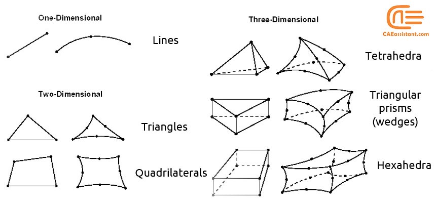
Figure 6: Mesh geometries for different solution spaces
5. Meshing methodologies: Top-down mesh versus Bottom-up mesh
There are two meshing methodologies available in Abaqus/CAE:
- Top-down mesh.
- Bottom-up mesh.
Top-down meshing relies on the geometry of a part to define the outer bounds of the mesh. You can use top-down meshing techniques to mesh one-, two-, or three-dimensional geometry using any available element type. The top-down mesh matches the geometry and this rigid conformance to geometry makes top-down meshing predominantly an automated process but may make it difficult to produce a high-quality mesh on regions with complex shapes. you may need to simplify and/or partition complex geometry so that Abaqus/CAE recognizes basic shapes that it can use to generate a high-quality mesh.
Bottom-up meshing uses the part geometry as a guideline for the outer bounds of the mesh, but the mesh is not required to conform to the geometry. Removing this restriction gives you greater control over the mesh and allows you to create a hexahedral or hexahedral-dominated mesh.
5.1. Top-down mesh or bottom-up mesh: Which suits your model better?
You can use bottom-up meshing techniques to mesh only solid three-dimensional geometry using all—or nearly all—hexahedral elements. It provides you with the most control over the mesh, However, you must also decide whether the resulting mesh is a suitable approximation of the geometry.
Loads and boundary conditions are applied to geometry. Therefore, you should check that the mesh is correctly associated with the geometry in bottom-up mesh in areas where they are applied. Proper mesh-geometry association will ensure that they are correctly transferred to the mesh during the analysis. See figure 7 to see An example of a bottom-up meshed part.
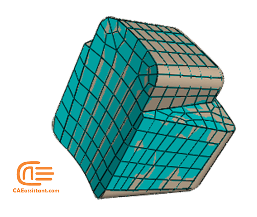
Figure 7: An example of a bottom-up meshed part
As you can see in figure 7, Abaqus/CAE displays bottom-up meshed regions using a mixture of the region geometry color (light tan) and the mesh color (light blue) to emphasize that the geometry and mesh may not be associated. Displaying both the geometry and the mesh allows you to view and edit the mesh-geometry associativity.
Since bottom-up meshing is a manual process that can be very time-consuming, it is recommended that you use this method only when the top-down methods fail to produce a satisfactory mesh.
6. Different Abaqus meshing techniques
After you have decided which methodology to use for your model, you choose the meshing technique, element shape, and some other properties for assigning to your model elements. You can see some of these options in the figure below which are available at “Assign Mesh Controls” (see figure 8) in the mesh module toolbox (Abaqus meshing techniques).
Free, Structured, and Sweep are the available techniques for top-down methodology. These techniques and their geometry requirements are well-defined, and loads and boundary conditions applied to a part are associated automatically with the resulting mesh. You may have a mixture of these top-down meshing techniques in your model which will be known as “Multiple”.
If you select the bottom-up technique, then you must use “Create bottom-up mesh” from the mesh module toolbox to create the mesh for your model manually by different methods shown in figure 9.
Another one??!! You don’t get tired, do you? Did you know most of the meshing we do is the Top-down meshing technique!! Remember you can get rid of meshing problems once and for all: “Different Techniques for Meshing in Abaqus“
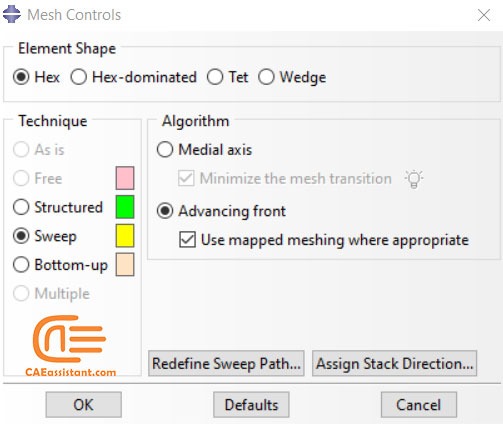
Figure 8: Mesh control in Abaqus mesh module
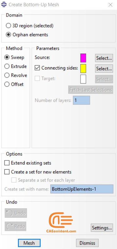
Figure 9: Create bottom-up mesh in the Abaqus mesh module
6.1. Abaqus free mesh
Free meshing uses no preestablished mesh patterns. It is impossible to predict a free mesh pattern before creating the mesh. Because it is unstructured, free meshing allows more flexibility than structured meshing. The topology of regions that you mesh with the free mesh technique can be very complex.
You can use this technique to mesh a region with the Tri, Quad, or Quad-dominated element shape options for two-dimensional regions. You can use the Tet element shape option for three-dimensional regions.
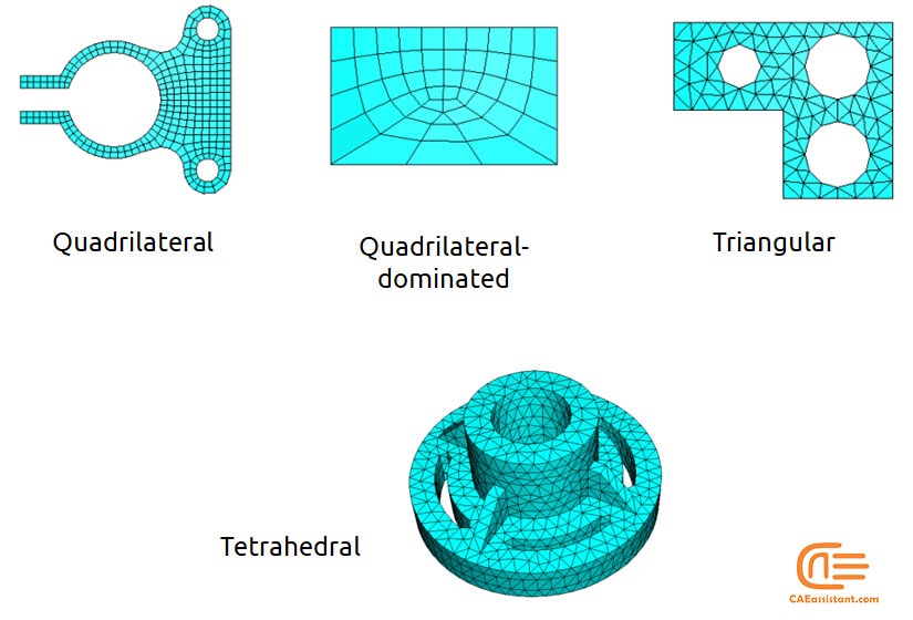
Figure 10: Element shapes for Free meshing
6.2. Abaqus structured mesh
The structured meshing technique generates structured meshes using simple predefined mesh topologies. Abaqus/CAE transforms the mesh of a regularly shaped region, such as a square or a cube, onto the geometry of the region you want to mesh. In general, structured meshing gives you the most control over the mesh that Abaqus generates.
Figure 11 illustrates how simple two-dimensional mesh patterns for triangles, squares, and pentagons are applied to more complex shapes.
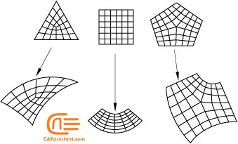
Figure 11: Simple 2D mesh patterns transformation for application in complex geometries
Figure 12 shows the regions that can be meshed using the structured meshing technique in 3D. Meshing more complex regions with structured technique may require manual partitioning. If you do not partition a complex region, your only meshing option may be the free meshing technique with tetrahedral elements.
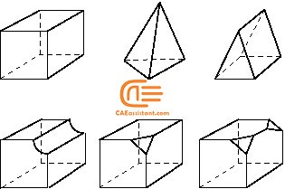
Figure 12: 3D Regions that can be meshed using the structured meshing technique
6.3. Abaqus swept mesh
Abaqus/CAE uses swept meshing to mesh complex solid and surface regions. The swept meshing technique involves two phases:
- Abaqus creates a mesh on one side of the region, known as the source side.
- Abaqus copies the nodes of that mesh, one element layer at a time, until the final side, known as the target side, is reached.
The face that connects the source side to the target side is called a connecting side. Abaqus copies the nodes along an edge, and this edge is called the sweep path. The sweep path can be any type of edge—a straight edge, a circular edge, or a spline. If the sweep path is a straight edge or a spline, the resulting mesh is called an extruded swept mesh. If the sweep path is a circular edge, the resulting mesh is called a revolved swept mesh.
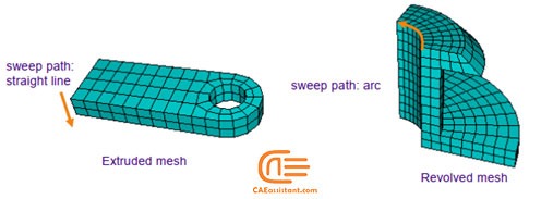
Figure 13: Extruded and Revolved Swept mesh
For example, figure 14 shows an extruded swept mesh. To mesh this model, Abaqus/CAE first creates a two-dimensional mesh on the source side of the model. Next, each of the nodes in the two-dimensional mesh is copied along a straight edge to every layer until the target side is reached.
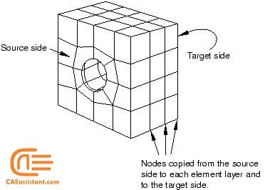
Figure 14: The swept meshing technique for an extruded solid
If the region can be swept in more than one direction, Abaqus/CAE may generate a very different two-dimensional mesh on the faces that it can select as the source side. As a result, the direction of the sweep path can influence the uniformity of the resulting three-dimensional swept mesh.
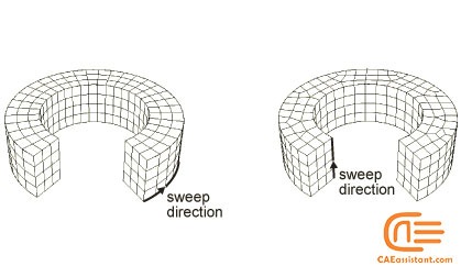
Figure 15: Effect of sweep path on the resulting swept mesh
6.4. Abaqus Bottom-up mesh
You can apply bottom-up meshing to any solid region, including regions that can be meshed using the top-down techniques, and to meshes that do not have any associated geometry. Once Abaqus has generated a bottom-up mesh, you need to evaluate whether it is suitable for the analysis and, if the geometry is present, verify that the mesh is correctly associated with it.
Each application of the bottom-up meshing technique involves four phases:
1. Selecting the domain within which Abaqus/CAE will create the mesh. You can choose either a three-dimensional geometry region or orphan elements.
2. Choosing the method that Abaqus/CAE will use to create the mesh. You can choose from the following methods:
- Sweep
- Extrude
- Revolve
- Offset (available only for orphan element selections)
3. You select the side, called the source side, that Abaqus/CAE will use to create a two-dimensional mesh to be swept, extruded, or revolved to fill a three-dimensional region.
4. You select the remaining parameters to complete the definition of the bottom-up mesh. For example, if you chose the sweep method, you can choose connecting sides and a target side.
These four phases are indicated on the Abaqus “Create bottom-up mesh” window in figure 16.
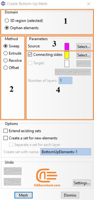
Figure 16: Bottom-up mesh generation phases
After we got familiar with different meshing techniques, we headed back towards some other terms that you need to know in meshing procedures.
6.5. Compatible mesh
Compatibility means that the element faces or element edges of the meshes of adjacent part instances share the same nodes and have the same topology at the common interface.
If you require mesh compatibility between two or more instances, you can do one of the following:
- Create a single part that contains all the bodies so that multiple instances are not necessary.
- Assemble instances of the parts in the Assembly module and use the Merge/Cut tool to merge the instances into a single instance. If you need to maintain the concept of separate part instances, you can create a partition at the common interface of the merged instances.
- If you must use separate parts, you can use tied contact to avoid the issue of mesh compatibility. Keep in mind that this is not true compatibility, and the accuracy of the solution may suffer.
7. What is Abaqus Adaptive mesh?
Nonlinear simulations often involve dramatic twists and turns, with structures undergoing large deformations or materials experiencing significant loss. This can wreak havoc on a static mesh, causing elements to become severely distorted and throwing off your results. Here’s where Abaqus adaptive mesh steps in to save the day.
Imagine a mesh that can adapt on the fly. Abaqus adaptive mesh is a powerful tool that automatically refines the mesh throughout your analysis. Think of it like constantly smoothing out wrinkles in a cloth – it maintains good mesh quality, ensuring your results stay accurate.
- Adaptive meshing is available for all first-order, reduced-integration continuum elements.
- Consists of two main tasks: creating a new mesh and remapping solution variables from the old mesh to the new mesh via advection.
- New mesh creation occurs at specified frequencies.
- Nodes are iteratively moved to smooth the mesh while retaining the initial gradation.
Just remember, Adaptive meshing is available only in ABAQUS/Explicit.
7.1. Adaptive meshing applications
Adaptive meshing is useful in a variety of applications:
- Transient Analysis: Dynamic impact, penetration, sloshing, forging
- Steady-State Processes: Extrusion, rolling
- Combination: Analyzing transient phases in steady-state processes
7.2. Basics of Adaptive meshing
- Adaptive meshing in ABAQUS/Explicit uses the Arbitrary Lagrangian-Eulerian (ALE) method.
- Regular intervals of mesh smoothing reduce element distortion and maintain good element aspect ratios.
- Mesh topology remains unchanged; the number of elements and nodes, and their connectivity, do not alter.
- Suitable for both Lagrangian (transient) and Eulerian (steady-state) problems.
7.3. Arbitrary Lagrangian-Eulerian (ALE) Method
- Lagrangian: Nodes move with material points, facilitating easy tracking of free surfaces and boundary conditions, but the mesh distorts with high strain gradients.
- Eulerian: Nodes remain fixed while material flows through the mesh, preventing mesh distortion but complicating free surface tracking.
- ALE: Mesh motion is constrained to material motion only where necessary, allowing independent motion otherwise.
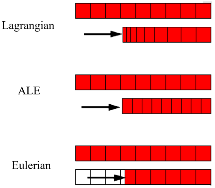
Figure 17: Motion of mesh and material with various methods
8. Adaptive Meshing in Practice: ALE simulation of an axisymmetric forging problem
Now, let’s make an example to understand the Abaqus Adaptive Meshing capability.
By using the adaptive meshing capability, a high-quality mesh can be maintained throughout the entire forging process.
Consider a forging process like in figure 18. Without adaptive meshing the results would be like figure 19 (a); but if we use adaptive meshing capability, the results are like figure 19 (b).
In figure 20, nodes along free boundaries move with material normal to the surface, adapting their position tangentially. Also, Interior nodes adaptively adjust in all directions.
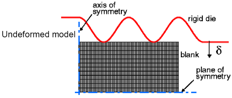
Figure 18: Forging process
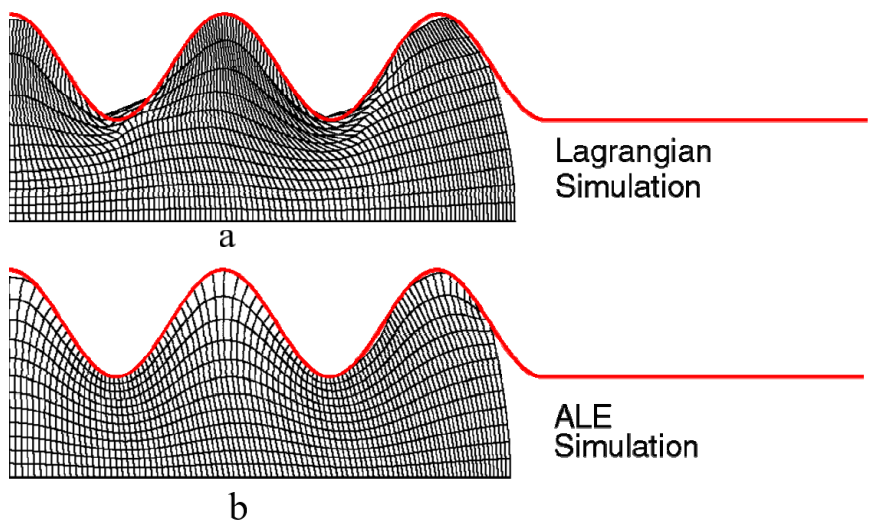
Figure 19: Lagrangian and ALE methods
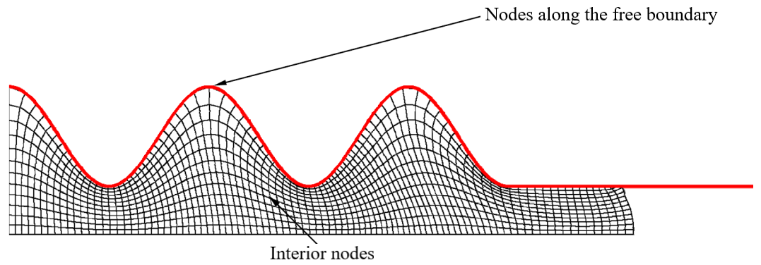
Figure 20: Free boundary and interior nodes
In a transient (Lagrangiantype) problem, such as this forging simulation, minimal additional input is required to invoke the adaptive meshing capability (figure 21).
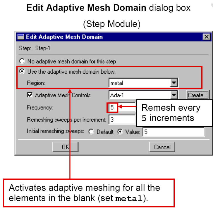
Figure 21: Adaptive meshing settings
9. Native and Orphan Abaqus mesh
A mesh generated for a geometric part in Abaqus/CAE will maintain its association with the parent geometry is called a native mesh.
An existing mesh can be imported from:
- Abaqus input (.inp) file
- Abaqus output database (.odb) file
- Nastran bulk data (.bdf) file
- ANSYS input (.cdb) file
- STL file (via plug-in)
An imported mesh is called an orphan mesh because it has no associated parent geometry. You can also create an Abaqus mesh part from selected part instances that you have meshed. An Abaqus mesh part contains no feature information and is defined by a collection of nodes, elements, surfaces, and sets.
Sets, surfaces, and section assignments are copied from the source parts or part instances when you create an Abaqus mesh part, so loads and interactions applied to the original parts are also applied to the Abaqus mesh part. You can add geometric features to a mesh part, and you can use the mesh editing tools to modify its nodes and elements.
10. How to convert Abaqus orphan mesh to geometry?
To convert an Abaqus orphan mesh to geometry, first, we need to import a part from an ODB (output database) file. This ODB file can be obtained from a previous simulation where the model was solved with an orphan mesh. In Abaqus, go to File > Import from Database > select ODB from the dropdown menu > choose the desired ODB file > click Continue.
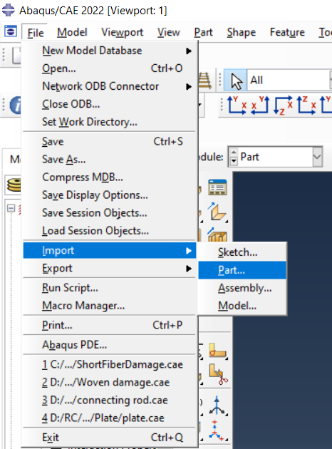
Figure 22: Import part from ODB
After importing the part from the ODB file, we will now change the orphan mesh to a regular part using Python commands. These commands allow us to automate the process and make it easier to work with the model. In the Part module, go to File > Import > Part and select the imported part from the ODB file. In the Name field, give a new name to the part, for example, “blank”. This will create a new part named “blank” with all its features and boundary conditions.
Next, we will use Python commands to convert this blank part from orphan mesh to a 2D regular part. In the Abaqus command line interface, type “Blank = mdb.models[‘Model-1’].parts[‘BLANK’]” and press Enter. This will assign the blank part to a variable named “Blank”.
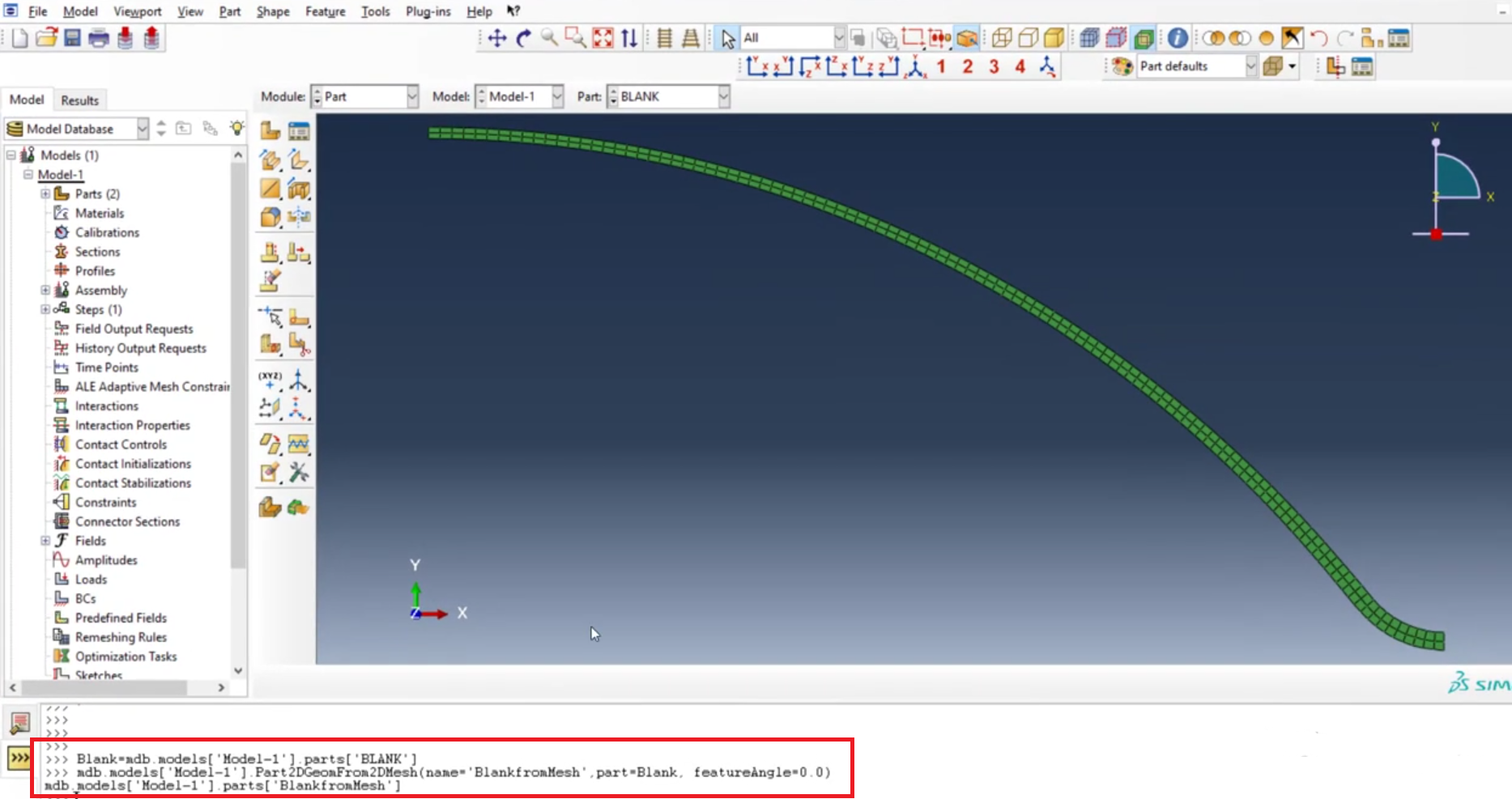
Figure 23: Orphan mesh
In the next command, we will use the “Part2DGeomFrom2DMesh” function, which takes in three arguments – name, part, and feature angle. In the “name” argument, enter a name for the new regular part, for example, “BlankfromMesh”.
In the “part” argument, enter the variable name we defined in the previous command, i.e., “Blank”. Lastly, in the “feature angle” argument, enter a value that controls the smoothness of the final part. A value of 0 means a very smooth part, while higher values result in a more jagged edge.
After executing this command, we will have a new 2D regular part named “BlankfromMesh” in the model database. This new part will have all its features and boundary conditions transferred from the previous blank part with an orphan mesh.
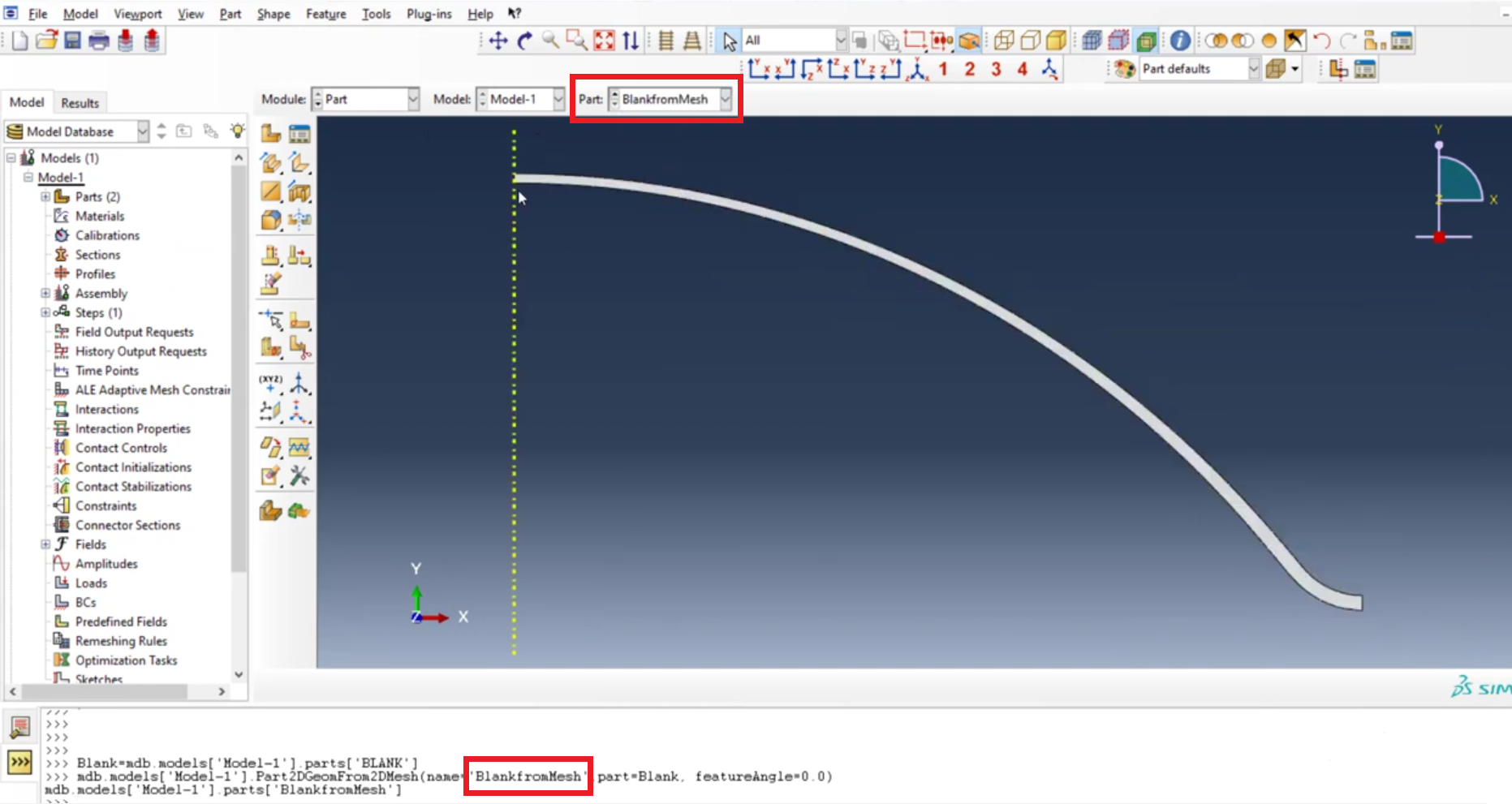
Figure 24: Real part
If you need more info, watch this video: https://www.youtube.com/watch?v=zF8Z9J1t50E
11. Verify Mesh
Upon completion of a meshing operation, Abaqus/CAE highlights any bad elements in the mesh. Abaqus also provides a set of tools in the Mesh module that allow you to verify the quality of your Abaqus mesh and obtain information about the nodes and elements in the mesh. You can use these tools to isolate regions where the mesh quality is poor and to guide you if you need to refine your mesh.
You can use the Analysis checks to verify that the elements in your mesh will pass the element quality checks that are included with the input file processor in Abaqus/Standard or Abaqus/Explicit. Abaqus highlights any elements that fail the mesh quality tests and displays the number of elements tested along with the number of errors and warnings in the message area.
11.1. Shape metrics
You can use the Shape metrics to highlight elements of a selected shape that do not meet one of the following selection criteria:
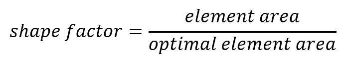
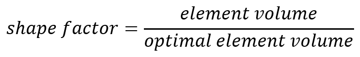
- Shape factor:
Abaqus highlights elements with a normalized shape factor smaller than a specified value. The shape factor criterion is available only for triangular and tetrahedral elements. The shape factor ranges from 0 to 1, with 1 indicating the optimal element shape and 0 indicating a degenerate element. Read More
11.2. Size metrics
You can use the Size metrics to highlight elements that do not meet one of the following selection criteria.
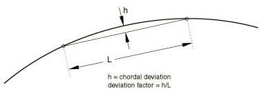
- The geometric deviation factor:
This factor is a measure of how much an element edge deviates from the original geometry, and Abaqus calculates this value by dividing the maximum gap between an element edge and its parent geometric face or edge by the length of the element edge. By default, Abaqus highlights elements whose geometric deviation factor is greater than 0.2. Abaqus calculates the geometric deviation factor only for elements in a native mesh. Read More
11.3. Analysis checks
Elements that will produce errors or warnings in the analysis can be highlighted. Abaqus highlights elements that fail the element checks specified in the Shape Metrics or Size Metrics tabbed pages as warnings. In addition, you can highlight any elements that generated errors or warnings using the checks found in the input file processor in Abaqus/Standard and Abaqus/Explicit in the appropriate colors.
Analysis checks are not currently supported for beam, gasket, and cohesive elements.
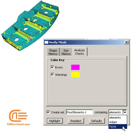
Figure 26: An example of mesh verification using Analysis checks
12. Summary
The importance of mesh in FEM is not negligible. It is a critical step in the FEM process, as the quality of the mesh directly affects the accuracy and efficiency of the solution. In this article, we learned the fundamentals of the Abaqus mesh, the Abaqus meshing methodologies which are Top-down mesh and Bottom-up mesh, and Abaqus meshing techniques to get one more step closer becoming a well-trained FEA analyst.
13. Users ask these questions
Now, let’s see some questions, which users asked us in social media and we have answered them.
I. Mesh of pipe elbow contain internal corrosion defect
Q: I want to mesh a pipe elbow contain a single defect in internal wall of extrados by mesh hexa or hexa deminate but i can’t do.
I used the method of partition but no result,please help me.
Thank you.
A: Fix your geometry and make it simple. I had the same problem but with extrados. Read this article to understand the meshing techniques or you can fix your meshing problem once and for all with this tutorial package: “Abaqus meshing techniques tutorial“.
This package introduces different meshing techniques in Abaqus. In finite element analysis, a mesh refers to the division of a physical domain into smaller, interconnected subdomains called elements. The purpose of meshing is to approximate the behavior of a continuous system by representing it as a collection of discrete elements. Meshing is of utmost importance in finite element analysis as it determines the accuracy and reliability of the numerical solution. Through this tutorial, initially, the mesh and related terms associated with meshing are declared. Abaqus mesh module and meshing process are introduced. Then, two different meshing methodologies: Top-down and Bottom-up with meshing techniques available for each one of them are completely explained. Some of the advanced meshing techniques and edit mesh toolset are also included. The consideration of mesh verification as the final step in the meshing process, along with its criteria, is undertaken. All the tips and theories determined in this tutorial are implemented in Abaqus/CAE as a workshop to mesh several parts. This package intends to take your ability to mesh different parts to a higher level.
It would be helpful to see Abaqus Documentation to understand how it would be hard to start an Abaqus simulation without any Abaqus tutorial.
One note, when you are simulating in Abaqus, be careful with the units of values you insert in Abaqus. Yes! Abaqus don’t have units but the values you enter must have consistent units. You can learn more about the system of units in Abaqus.