The A to Z of Buckling: Column Buckling, Buckling Equations, and More
Buckling is a structural phenomenon that occurs when a component subjected to some forces deforms suddenly in a lateral direction. This lateral deformation significantly reduces the component’s stiffness and load-carrying capacity, often rendering it ineffective for its intended purpose. While buckling doesn’t always involve material failure, it represents a critical form of instability that engineers must carefully address.
Understanding and analyzing buckling is vital in structural engineering because it directly impacts the safety and performance of structures like columns, beams, and braces. Accurately predicting when and how buckling occurs allows engineers to design more reliable systems. Software tools like Abaqus are invaluable for performing buckling analysis, enabling precise modeling of this complex behavior.
In this blog, we will first explore the different types of buckling and the critical factors influencing its occurrence. Then, we’ll guide you through how to perform linear and nonlinear buckling analysis using Abaqus, with step-by-step examples. By the end, you’ll gain a clear understanding of buckling behavior and how to use Abaqus effectively to ensure structural stability in your designs.
|
You can learn Abaqus from the very beginning with the package below: |
All about buckling analysis, practical examples to learn the buckling error-free in Abaqus. |
1. What is Buckling?
Buckling refers to a type of structural instability in which a structural member, under compressive loads or other forms of loading, experiences a sudden lateral deformation. This deformation can lead to a significant reduction in the stiffness of the member and drastically decrease its load-carrying capacity. This phenomenon does not necessarily result in material yielding or fracture, but it is considered a failure mode because, after this, the member loses its ability to support any load.
For example, buckling can occur in compressive members like columns, beams subjected to lateral loads, or even in structures exposed to bending or torsional loading.
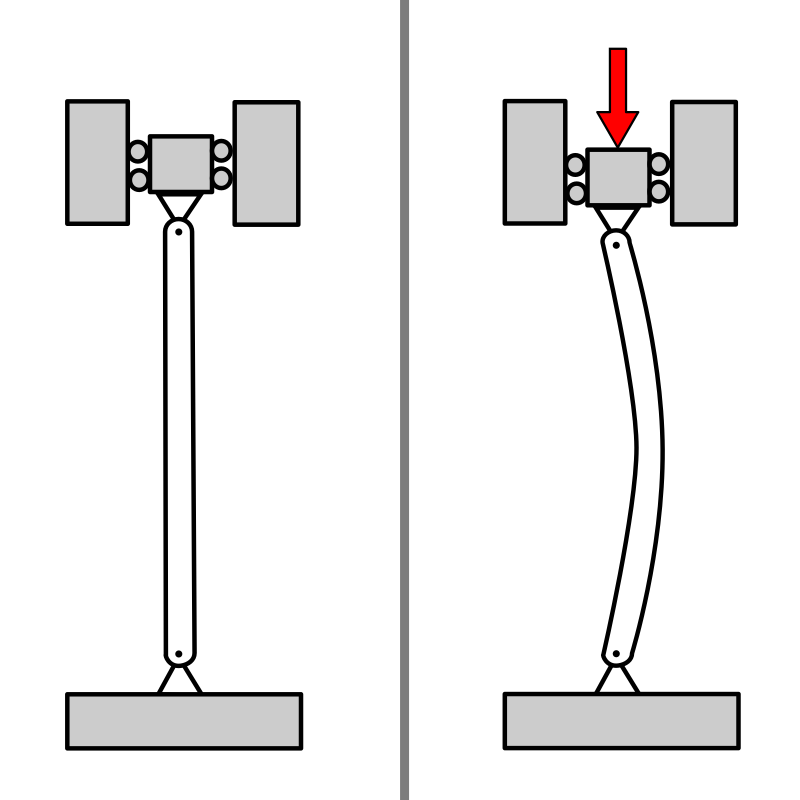
Figure 1: A depiction of buckling
2. Types of Buckling in Structural Engineering
Buckling can manifest in various forms depending on the type of loading, structural member geometry, and boundary conditions. Understanding the different types of it is essential for accurately analyzing and preventing failures in structures. In this section, we will explore the main categories of buckling, which include:
2.1. Global buckling
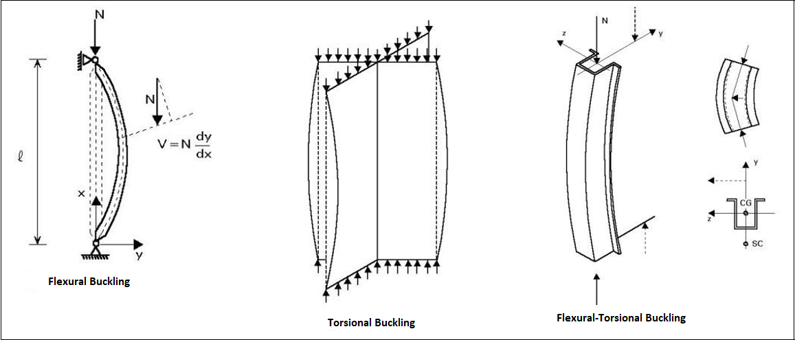
This phrase refers to the instability and failure of a structural member due to lateral deformations caused by compressive loads. This condition can manifest in three different forms: flexural buckling, torsional buckling, and flexural-torsional buckling, which will be discussed in the following sections. In this category, the overall lateral stability of the structure is compromised due to compressive stresses.
|
🎙️ Prefer Listening Over Reading? 🎙️ In our latest podcast episode, we cover everything from what buckling is to how it’s analyzed in Abaqus—all in one concise audio guide. Whether you’re curious about the fundamentals of buckling or looking to understand its application in Abaqus, this episode brings it all together in an engaging and easy-to-follow format. 👉 Click [here] to listen now!Tune in and get a clear insight into buckling without reading the entire article. |
2.1.1 Flexural Buckling
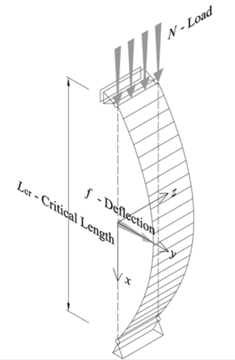
This type is characterized by deformation due to bending, which typically occurs around the axis with the highest slenderness ratio—usually the weaker axis of the section or the one with the smaller radius of gyration. Members subjected to different types of loading, regardless of their shape, can experience this form of buckling.
Figure 2: Flexural Buckling [ref]
2.1.2. Torsional Buckling
Torsional buckling occurs when a structural member fails due to twisting around its longitudinal axis. This failure mode is common in members under compressive loads where the entire section rotates or twists as a whole. Typically seen under pure compression loads where a significant component of torsional stress is present. Most prone in open cross-sections, such as channels or angles, and can occur in doubly symmetric shapes like I-beams when conditions favor torsional instability.
2.1.3. Flexural-Torsional Buckling
A more complex mode combining lateral bending and twisting, flexural-torsional buckling involves both the bending of a member and its simultaneous twisting. It often resembles lateral-torsional buckling observed in unbraced beams but applies specifically to compression members. Occurs under axial compression, especially when the centroid and shear center of the cross-section do not align. It affects non-doubly symmetric cross-sections, such as channels, angles, and some types of beams. Doubly symmetric sections (e.g., wide flange sections) typically experience simpler torsional or flexural buckling rather than this combined mode.
Figure 3: Types of global buckling [Ref]
2.2. Local Buckling
In local buckling, only a portion of the member subjected to buckles and loses its load-bearing capacity, often due to the slenderness of that specific part of the member. Local buckling can occur under both distributed and concentrated loads. In this type, the axis of the member does not deform, but the cross-section of the beam buckles significantly reduces the load-carrying capacity of the affected area. In this case, the overall stability of the structure may not be compromised.
Figure 4: a) global buckling b) local Buckling [Ref]
2.3. Elastic Buckling
Elastic Buckling occurs when a structure deforms elastically (reversibly) under various types of loading. In this state, the structure returns to its original shape once the load is removed. This type is commonly observed in metallic structures and those exhibiting elastic behavior. Euler’s formula for determining the critical buckling load is one of the most important equations in this field.
2.4. Plastic Buckling
Plastic Buckling occurs when a structure undergoes plastic (irreversible) deformation under various types of loading. In this type of buckling, permanent deformation is induced in the structure, and once the load is removed, the structure does not return to its original state. This form of buckling is typically observed in concrete structures or those operating in the plastic region.
 |
⭐⭐⭐ Free Abaqus Course | ⏰10 hours Video 👩🎓+1000 Students ♾️ Lifetime Access
✅ Module by Module Training ✅ Standard/Explicit Analyses Tutorial ✅ Subroutines (UMAT) Training … ✅ Python Scripting Lesson & Examples |
Note: There are examples of buckling in our Buckling tutorial package. It teaches you step by step how to do an Abaqus buckling. Of course you can find other stuff and examples in this blog for free.
3. When Does Buckling Occur?
In this section, we will first examine the parameters influencing buckling analysis, which include factors such as member length, support conditions, and cross-sectional geometry. Then, we will discuss the concept of critical buckling load and how it is calculated using Euler’s formula, along with its effects on the structural stability.
It is important to note that the taller and slimmer the member, the more susceptible it is to buckling. Various structural members such as columns, beam-columns, tie beams, and braces are prone to buckling. Structural engineers must perform accurate calculations and proper design of members against buckling to ensure that the structure remains safe under potential loads.
3.1. Parameters Influencing Buckling Analysis
The resistance of members to buckling depends on various factors such as the length, shape, cross-sectional area of the members, stiffness, support conditions, and so on. To account for these effects, parameters are defined that allow for the calculation of the critical buckling load based on the applied compressive force. The critical buckling load is the maximum load that a member can support without buckling.
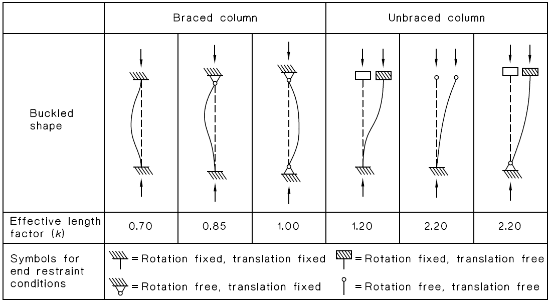
- Effective Length Factor
This parameter essentially reflects the length of the member where the risk of buckling is higher. As this length increases, the likelihood of buckling also rises. The effective length factor, commonly represented by the letter K depends on the support conditions at both ends of the member. It is worth noting that achieving ideal boundary conditions (such as perfectly rigid supports) is often impractical in reality. Therefore, for design purposes, effective length factors are sometimes set higher than the theoretical values.
Figure 5: Approximate values of effective length factor k [Ref]
- Effective Length
The effective length is defined as the product of 𝐾 and the free span between supports (𝐿). This length represents the equivalent length of the member if it were constructed with pinned supports at both ends.
- Radius of Gyration
To better understand the concept of the radius of gyration and its effect on the stability of structures, we can explain it with a more tangible example.
Imagine a spinning top:
The faster it spins, the more stable it becomes and the less likely it is to tip over. One of the main reasons for this stability is how the mass of the top is distributed.
If the top has a heavy base with more mass concentrated near the bottom, it will be more stable. This is because the mass is closer to the surface it’s in contact with, making it more resistant to tipping.
If the top has a wider base, its stability also increases. This means it requires more force to tilt the top, and its center of gravity is positioned in a way that maintains its balance and rotation.
Now, let’s apply this concept to engineering structures like columns or beams. Columns are under compressive forces and might buckle due to sudden pressure (which means losing stability and rapidly deforming).
The radius of gyration can be seen as the “base” of the column:
A larger radius of gyration indicates that the cross-sectional area of the column is designed so that more material is distributed farther from the center. Just like a top with a wider base, the column becomes more resistant to lateral forces and buckling.
For example, if a column has a wider or better-distributed cross-section, it will be more stable and resist sudden deformations more effectively. Just like the top with a wider base is more stable and less likely to tip over, a column or beam with a larger radius of gyration is less prone to buckling.
In the end, the radius of gyration represents how the material in a structure is distributed to resist buckling. The larger the radius, the more efficiently the material is used, resulting in a structure that is better able to withstand destabilizing forces.
In fact, the larger the radius of gyration, the more stable the column is, just like a top with a wider base, making it less prone to tipping or sudden deformation.
When the radius of gyration is not equal about the two principal axes of a cross-section, the section tends to buckle around the weaker axis, which has the smaller radius of gyration.
The radius of gyration about the x-axis is calculated using the following formula:
The moment of inertia is a measure of an object’s resistance to rotational motion about a specific axis. It depends on the object’s mass distribution relative to the axis of rotation and is crucial in the study of dynamics, especially in the analysis of rotational systems.
- Slenderness Ratio
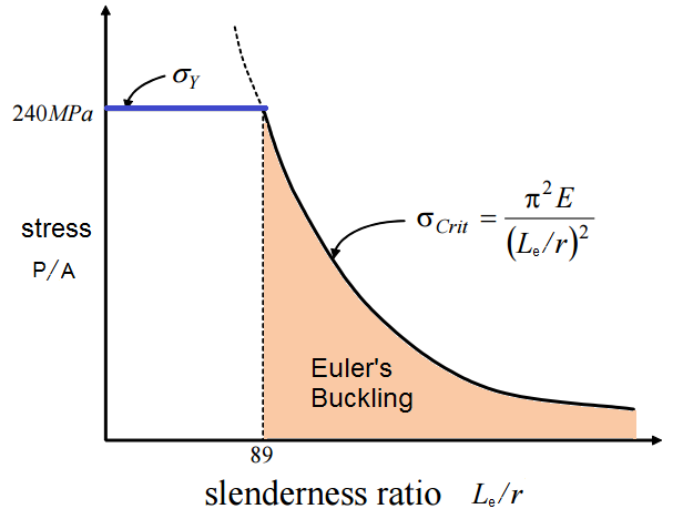
The slenderness ratio is defined as the ratio of the effective length of a member to the radius of gyration of its cross-section (KL/r). This parameter significantly influences the failure modes of a section. Based on the definition of the slenderness ratio, sections are categorized into three main types, which help in analyzing the behavior of sections under axial loading. These three categories are as follows:
- Short (Stocky) Sections: These sections have a low slenderness ratio, leading them to fail under compressive stress (yielding) without experiencing any buckling.
- Long (Slender) Sections: These sections generally fail due to buckling before reaching their yield strength. The behavior of such sections is influenced by their modulus of elasticity E.
- Intermediate Sections: Sections with a slenderness ratio between the short and long categories exhibit a failure mode that combines both buckling and compressive stress.
3.2. Critical Buckling Load
Imagine you have an aluminum pipe that is intended for use in constructing a radio tower. This pipe is positioned vertically, and a compressive load is applied from above, such as the weight of equipment or wind force. Initially, when a small load is applied to the pipe, it experiences linear compression and shrinks. However, as this load gradually increases, there will come a moment when the pipe suddenly deforms laterally and bends; this moment is precisely when the pipe can no longer withstand additional load. The load that leads to this instability and sudden deformation is called the critical buckling load.
As you can see, buckling can occur in various types of structures, but the most well-known and common example is the critical buckling load in columns. We will discuss this topic in detail in the next section.
4. Buckling of Columns | Column Buckling
Since columns are primary load-bearing elements of almost all types structure building and are directly subjected to compressive forces, the potential for column buckling must be thoroughly evaluated. Buckling can occur in both concrete and steel columns. In concrete columns, if longitudinal reinforcements are not properly secured, they may buckle, leading to a decrease in the column’s strength and ductility. To mitigate this risk, ties should be correctly placed at specified intervals to ensure all longitudinal reinforcements are properly braced, minimizing the chance of buckling.
The probability of buckling in concrete columns decreases with a larger cross-sectional area and improved seismic load-bearing performance. However, poor concrete quality can lead to concrete spalling around the reinforcements during seismic events, reducing its role in supporting gravity loads. In such cases, the gravity loads are primarily carried by the longitudinal reinforcements, and due to their slenderness, global buckling of the column may occur.
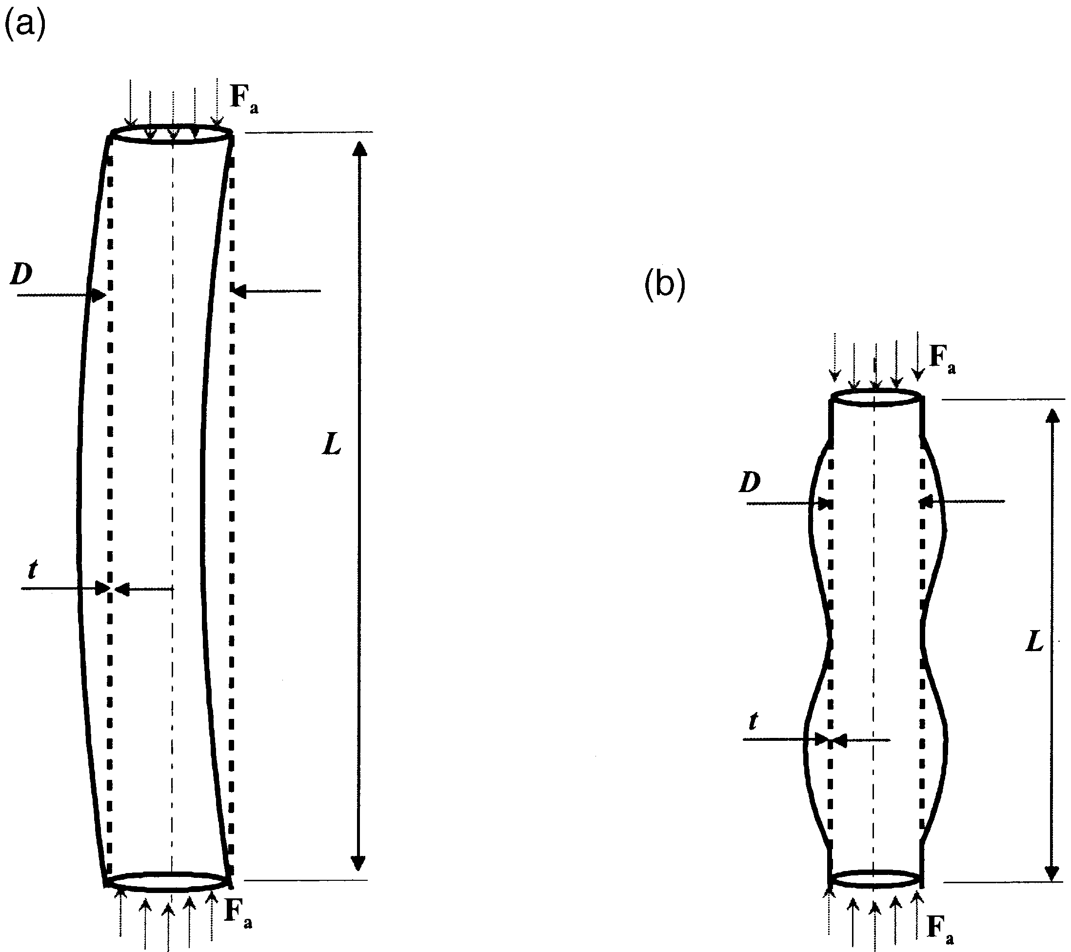
Figure 6: Buckling of Columns [Ref]
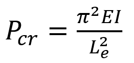
To calculate the critical load due to buckling in columns, you can use Euler’s formula (buckling euler) as follows:
Figure 7: Euler’s Buckling
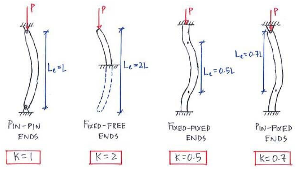
The length of the column that is placed between the supports and is less than the original length in some cases is called the effective length of the Le.
In the following, the general solving method of buckling equations, its usage in the finite element software and, different types of solving techniques and capabilities of the software to process buckling load in various structures is investigated.
So we’ve talked about columns and beams all along and about how they buckle; but what are these structures anyway? what are the differences between them, is it only buckling that annoys us in our analyses? All great questions which you can get all the answers in “Concrete Column Analysis + Beams Explained: Design, FEA” blog.
5. How to do Abaqus Buckling Analysis?
Buckling is a critical failure mode that occurs when a structure under loading becomes unstable, leading to sudden and potentially catastrophic deformation. Predicting the buckling behavior of a structure is essential to ensure safety and optimize design.
Abaqus provides powerful tools to perform buckling analysis using two distinct approaches: linear buckling analysis (also known as eigenvalue buckling) and nonlinear buckling analysis. Each method serves specific purposes and is suited for different types of structural behavior. Just note that if you want to do a nonlinear Abaqus buckling analysis, you have to do a linear analysis at first.
In the following sections, we’ll explore these two approaches in detail, focusing on their principles, applications, and how to perform them step by step in Abaqus.
5.1. Why Perform Both Linear and Nonlinear Buckling Analysis?
Linear buckling analysis provides a quick and conservative estimate of the critical load, assuming perfect geometry and linear elastic behavior. This makes it ideal for early-stage design and safety checks. However, real-world structures are rarely perfect and often experience nonlinear behavior before collapsing.
To capture the true behavior of a structure under loads, nonlinear buckling analysis is essential. It accounts for geometric imperfections, material yielding, and postbuckling stability, providing a realistic assessment of the structure’s collapse load.
Using both approaches ensures a safe and robust design, balancing computational efficiency with real-world accuracy.
6. Abaqus Linear Buckling
This guide focuses on the linear approach, which uses the “Buckle” step in Abaqus to estimate critical loads; it may be called “Eigenvalue buckling analysis”. In this analysis, Abaqus assumes that the structure behaves linearly elastic. This means the analysis only considers the linear stiffness of the material, and any nonlinear or inelastic material behavior (e.g., plasticity, creep, or viscoelasticity) is ignored. Therefore, the first thing we have learned here that for eigenvalue buckling (linear buckling), we only need to define Young’s modulus and Poisson’s ratio for material properties.
Elastic Behavior Assumption:
- Linear buckling assumes the structure behaves linearly elastic up to the point of buckling. This means the material follows Hooke’s Law (stress is proportional to strain) without yielding or undergoing permanent deformation.
- As a result, the analysis only focuses on the point where instability first occurs, without considering what happens afterward.
Critical Load as a Threshold:
- The critical buckling load predicted by linear analysis represents the point at which the structure’s stiffness matrix becomes singular (loses stability).
- This is the theoretical threshold beyond which the structure begins to deform in the predicted buckling mode shape.
Before Buckling:
- Since linear analysis does not account for postbuckling effects or imperfections, it only provides an upper bound or approximation of the load at which buckling begins.
6.1. What are Eigenvalue, Eigensolver and Mode Shape of Buckling?
An eigenvalue is a special number that represents a critical multiplier for the applied load pattern in the buckling analysis. The smallest eigenvalue corresponds to the critical load at which the structure is expected to buckle.
An eigensolver is a numerical algorithm used to compute eigenvalues and eigenvectors (mode shapes). Abaqus offers two eigensolvers:
- Subspace Iteration Method: Efficient for models requiring fewer eigenvalues.
- Lanczos Method: Faster for large systems with many degrees of freedom.
A buckling mode shape represents the shape a structure adopts at the point of instability. Each eigenvalue has a corresponding mode shape that shows how the structure deforms when it buckles. Mode shapes are relative, not absolute. In Abaqus, they are normalized so the largest displacement component is 1.0. They show patterns, not magnitudes.
Note: Negative eigenvalues indicate that the structure could buckle if the load direction is reversed. For example, a plate under shear loading may have the same buckling load for positive and negative shear.
Here is the brief break down:
The eigenvalue buckling analysis solves the equation:
- Base stiffness (
): Stiffness matrix of the structure in its initial state.
- Eigenvalue (
): These are the eigenvalues (load multipliers) you are solving for. Each eigenvalue represents the factor by which the live load Q must be multiplied to reach a critical buckling state.
- Incremental Stiffness (
): This is the incremental stiffness matrix that arises from the live load pattern (Q) applied in the buckling step.
- Mode Shape or eigenvectors (
): These are the eigenvectors, which correspond to the buckling mode shapes. They show how the structure will deform (shape) at a given critical load.
- Incremental load pattern or the one you define in the Abaqus (Q): Q is the pattern of the load applied in the buckling step. It describes where and how loads are applied but not their absolute magnitude. For example, it could be a distributed pressure over a column or a point load at the tip of a cantilever beam.
6.2. How Abaqus operates and solve the linear buckling?
- Set the Base State (
):
- If there’s a preload (e.g., gravity load or thermal stress), perform a static analysis step first. This defines the base stiffness matrix
.
- If no preload exists,
corresponds to the stiffness of the undeformed structure.
- Define the Incremental Load Pattern (Q):
- In the “Buckle” step, define the pattern of the live load Q.
- Example: Apply a unit distributed pressure to a shell or a point load to a column. This serves as Q.
- Solve for Eigenvalues (
):
- Abaqus computes a set of eigenvalues using any eigensolver you choose (
) and their corresponding eigenvectors (
).
- Typically, you focus on the smallest eigenvalue (
), as it represents the first buckling mode.
- Interpret the Results:
- Compute the critical buckling load using:
- Visualize the mode shapes (
) in the Abaqus Visualization module to understand how the structure will deform.
We have explained an Euler beam in one of the lessons in our beginner package. The Euler beam is analyzed, and its buckling load is determined by solving the corresponding differential equations. Maybe this lesson will help you out to understand the mathematic behind the buckling analysis.
6. Step by step example for Linear Abaqus Buckling
Now, let’s solve a problem together in the Abaqus to see the linear Abaqus buckling in practice. As you know, solving a problem in Abaqus requires to go through the almost all modules of Abaqus from Part to visualization and the linear buckling is no exception.
1. Creating Geometry (Part module)
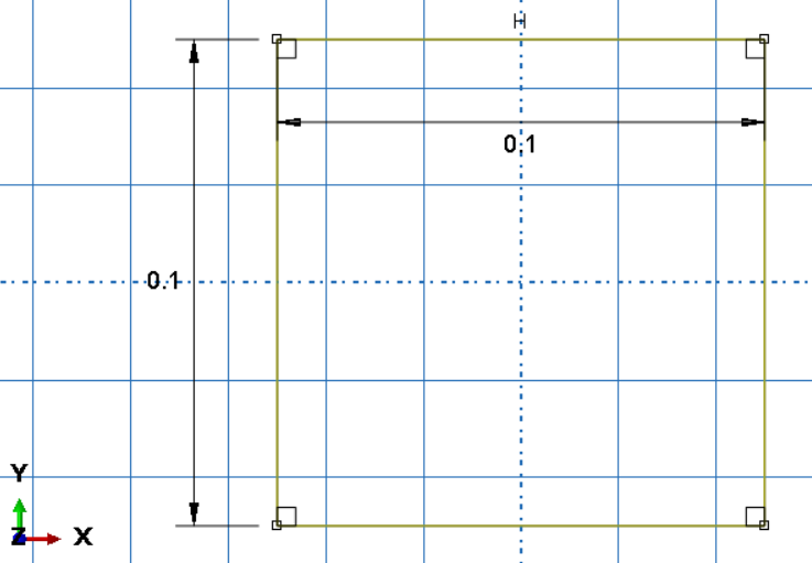
First, create a rectangular shell column with the dimensions below and extruded up to 45 cm.
Note: All units used in this simulation are SI (metric) units.
Figure 8: dimensions of the shell column
2. Material properties
As we said before, for Abaqus linear buckling analysis, we need only the Young’s modulus and Poisson’s ratio; therefore, we enter the 69 GPa and 0.3 for each one, respectively.
The thickness of the shell would be 2 millimeters.
3. Step
Because we only have one part, we just create instance from the part in the Assembly module and move to the Step module.
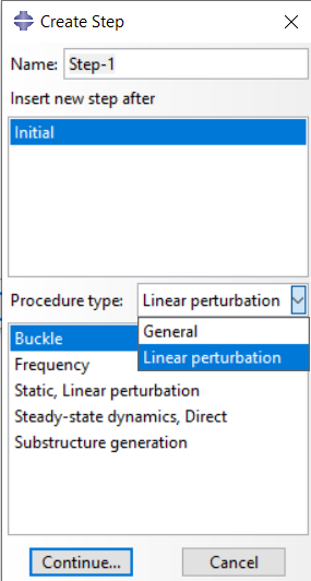
In the “Create Step” edit window, go the “Linear perturbation” category (fig 9) and select the step “Buckle”. Then, you must choose the eigensolver and determine the number of eigenvalues.
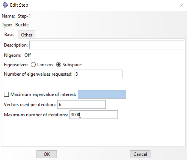
The “Subspace” eigensolver is selected by the default and we want to see the 3 mode shapes (fig 10). We increase the maximum number of iterations up to 3000 just in case.
Figure 9: selecting Buckle Step
Figure 10: determining the eigensolver and number of eigenvalues
4. Boundary Conditions and Loading
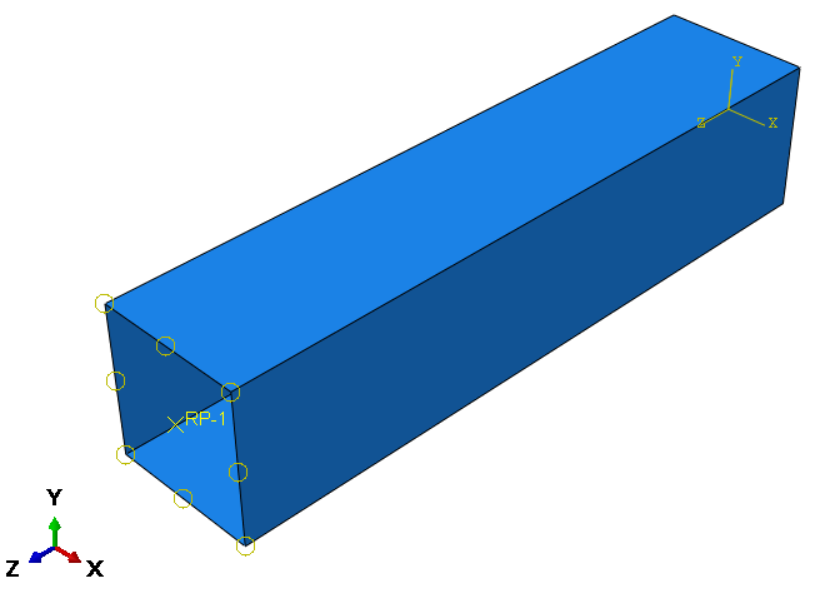
For this part, first, we create a reference point and make Tie constraint with the edge of the column according to the figure 11.
Figure 11: Reference point for boundary conditions and loading
Next, we fix the bottom of the column (U1 = U2 = U3 = 0) and all directions in the reference point (U1 = U2 = U3 = UR1 = UR2 = UR3 = 0) except U3. Then, we apply a concentrated force on the reference point in the -U3 direction.
5. Meshing and Running the problem
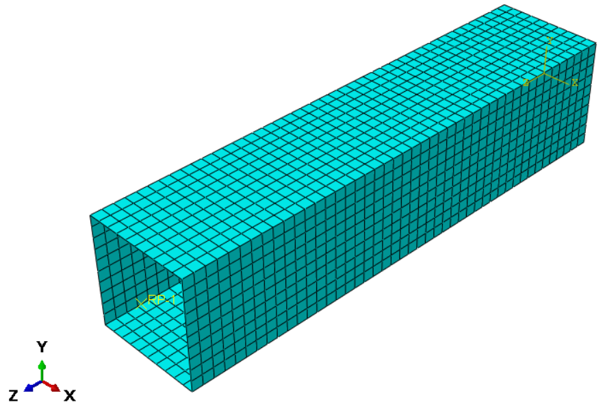
Finally, we mesh the model (fig 12) and in the Job module create a job for it and run the analysis.
Figure 12: Meshing the model
6. Results and Visualization module
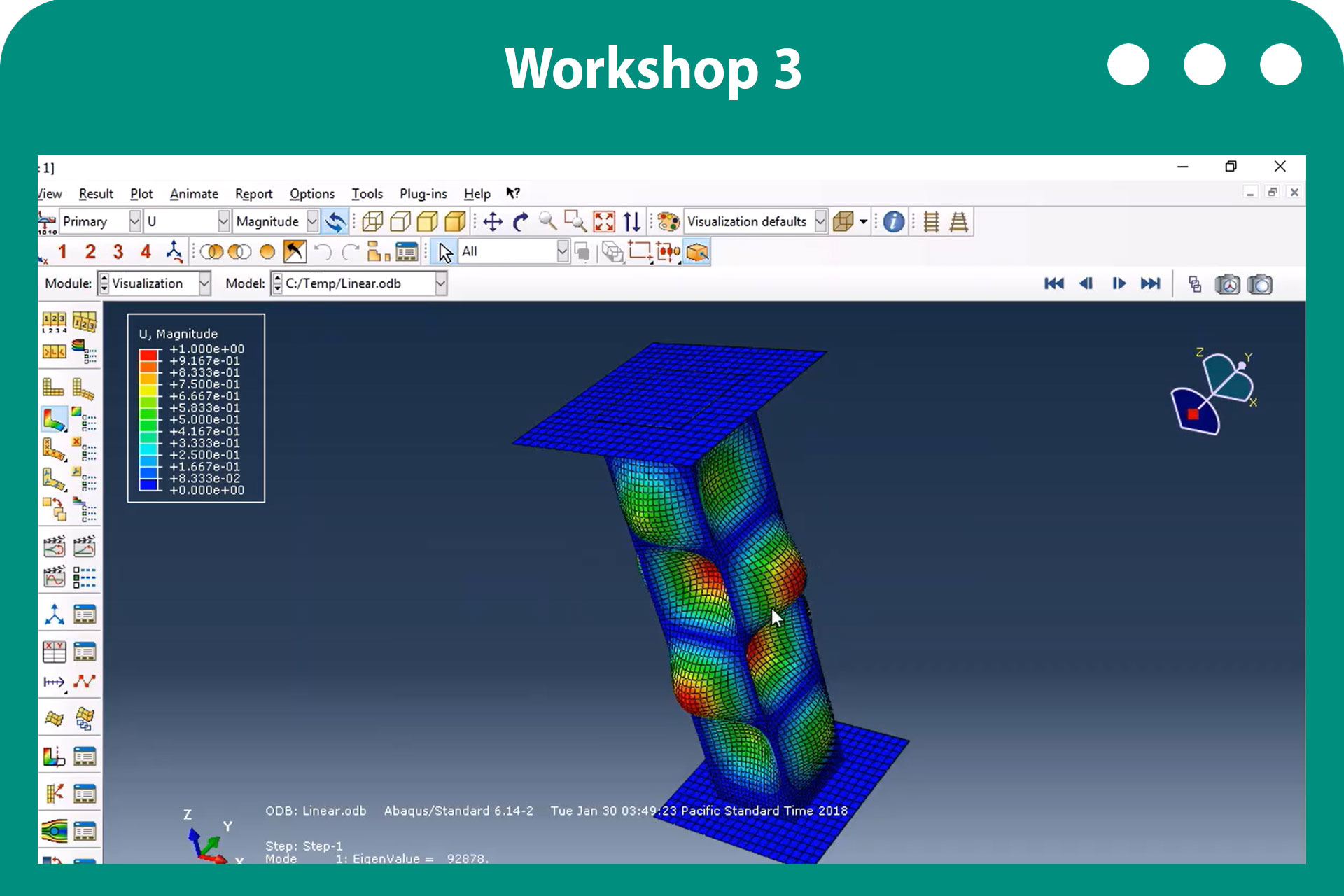
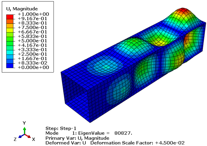
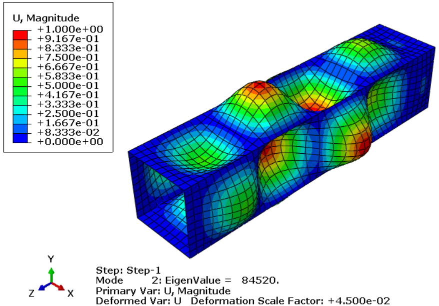
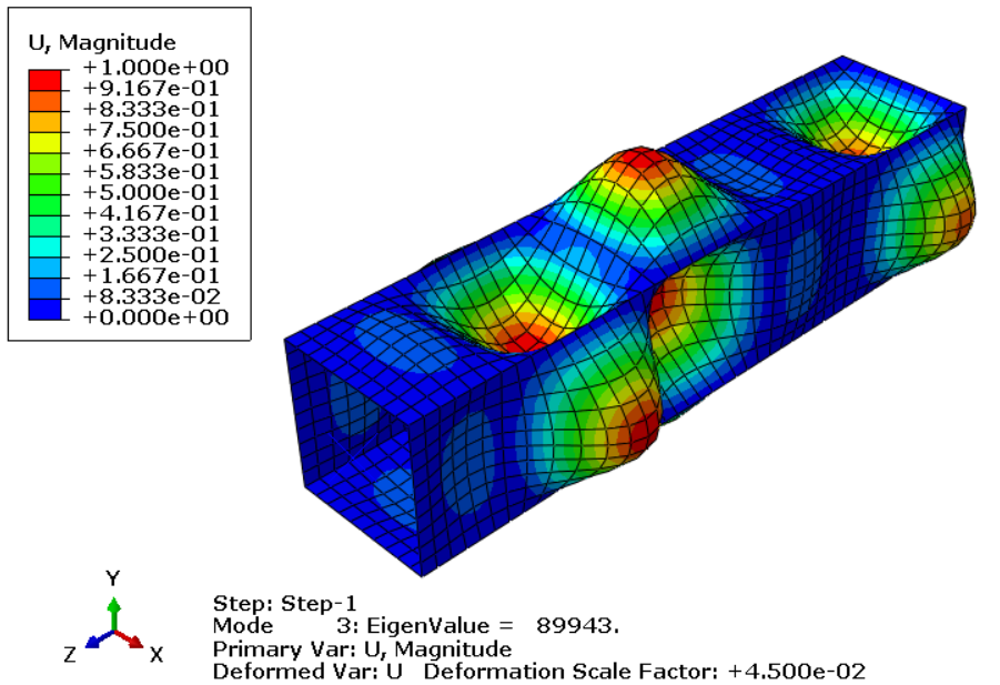
After the job is completed, go to the visualization module to see the results. You can see the 3 eigenvalues and 3 mode shapes of this shell column in the figures below.
Figure 13: First eigenvalue and mode shape
Figure 14: Second eigenvalue and mode shape
Figure 15: Third eigenvalue and mode shape
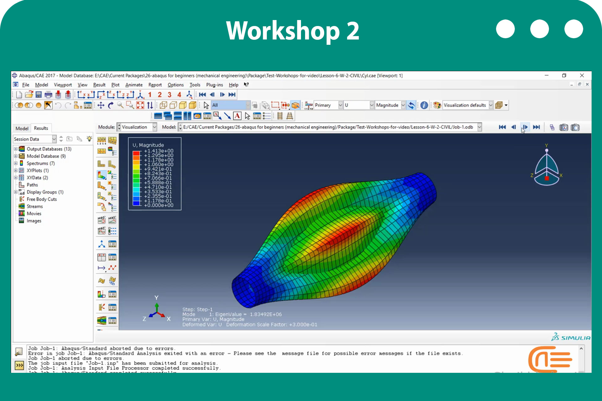
You can have the full tutorial of this example in the third workshop of our buckling tutorial in Abaqus.
7. Nonlinear Abaqus Buckling
As we said earlier, to capture behavior of structures in the real-world scenarios, we need nonlinear buckling to capture things like geometric imperfections, material yielding, and postbuckling stability. Added to the list that we have the challenges below as well.
When a structure buckles in the real world, the response often includes:
Unstable Behavior:
In a typical static analysis, the load is the driving parameter. You apply a specific load magnitude, and the solver calculates the resulting displacements. However, in nonlinear problems (like snap-through buckling or collapse):
- The load-displacement relationship is not linear.
- The structure may reach a point of instability, where increasing the load causes large displacements or even a load decrease (negative stiffness).
This creates a problem for traditional solvers because they rely on a predefined load progression. If the load decreases or the response becomes unstable, the solver can’t follow the correct solution path.
Imperfection Sensitivity:
Real structures are not perfect. Small imperfections in geometry can drastically affect the load at which buckling occurs.
Postbuckling Behavior:
After buckling, the structure’s response may stabilize (carry more load) or destabilize (collapse).
These behaviors cannot be captured by linear buckling analysis, so nonlinear techniques like the Riks method are needed.
The equilibrium path and where the analysis is completed
In nonlinear problems, the load-displacement curve can have regions where:
- The load decreases (snap-through or snap-back behavior).
- There’s no clear direction for the solver to follow if it relies only on load or displacement increments.
Traditional solvers struggle to follow this equilibrium path through unstable regions.
These behaviors and challenges cannot be captured by linear buckling analysis, so nonlinear techniques like the Riks method are needed.
7.1. How the Riks method overcome Nonlinear buckling challenges?
Unstable Behavior:
The method assumes that all loads are scaled proportionally. For example, if you apply a uniform pressure and a point force, both increase together according to a single scaling factor. The Riks method solves this by treating the load proportionality factor (𝜆) as an unknown variable. This means:
Instead of directly specifying the load magnitude, the Riks method scales the applied loads proportionally using 𝜆. The solver determines 𝜆 as part of the solution process, along with the displacements.
The total load at any point during the analysis is given by:
Where is the dead load (initial load applied before the Riks step),
is the reference load (the load pattern applied in the Riks step),
is the total load vector, and 𝜆 is the load proportionality factor. The Riks method solves for 𝜆 and the displacements simultaneously, allowing it to track the load-displacement response even in regions where the load decreases.
The equilibrium path and where the analysis is completed
Instead of moving directly along the load or displacement axis, the Riks method follows the curve using the arc length (𝑙). This helps the solver navigate through unstable regions, ensuring it doesn’t miss any part of the response.
Arc length is the geometric distance along the load-displacement curve. If you imagine the curve as a path, the arc length measures how far you’ve traveled along that path, regardless of whether the load or displacement is increasing or decreasing.
Here is an example to help you understand these concepts:
Think of solving the problem as navigating a winding, hilly trail:
- Load Proportionality Factor (𝜆): Determines the slope and adjusts your pace (how much effort/load to apply) to stay balanced and keep progressing.
- Arc Length (𝑙): Tracks how far you’ve traveled along the trail, ensuring you’re following the intended path and not going off course or getting stuck.
- End of the Solution: Happens when you reach the trail’s end (termination criteria), whether it’s a peak, a valley, or a specific waypoint.
The details of this procedure are beyond the scope of this blog, but if you need more information, you can read this in the Abaqus documentation.
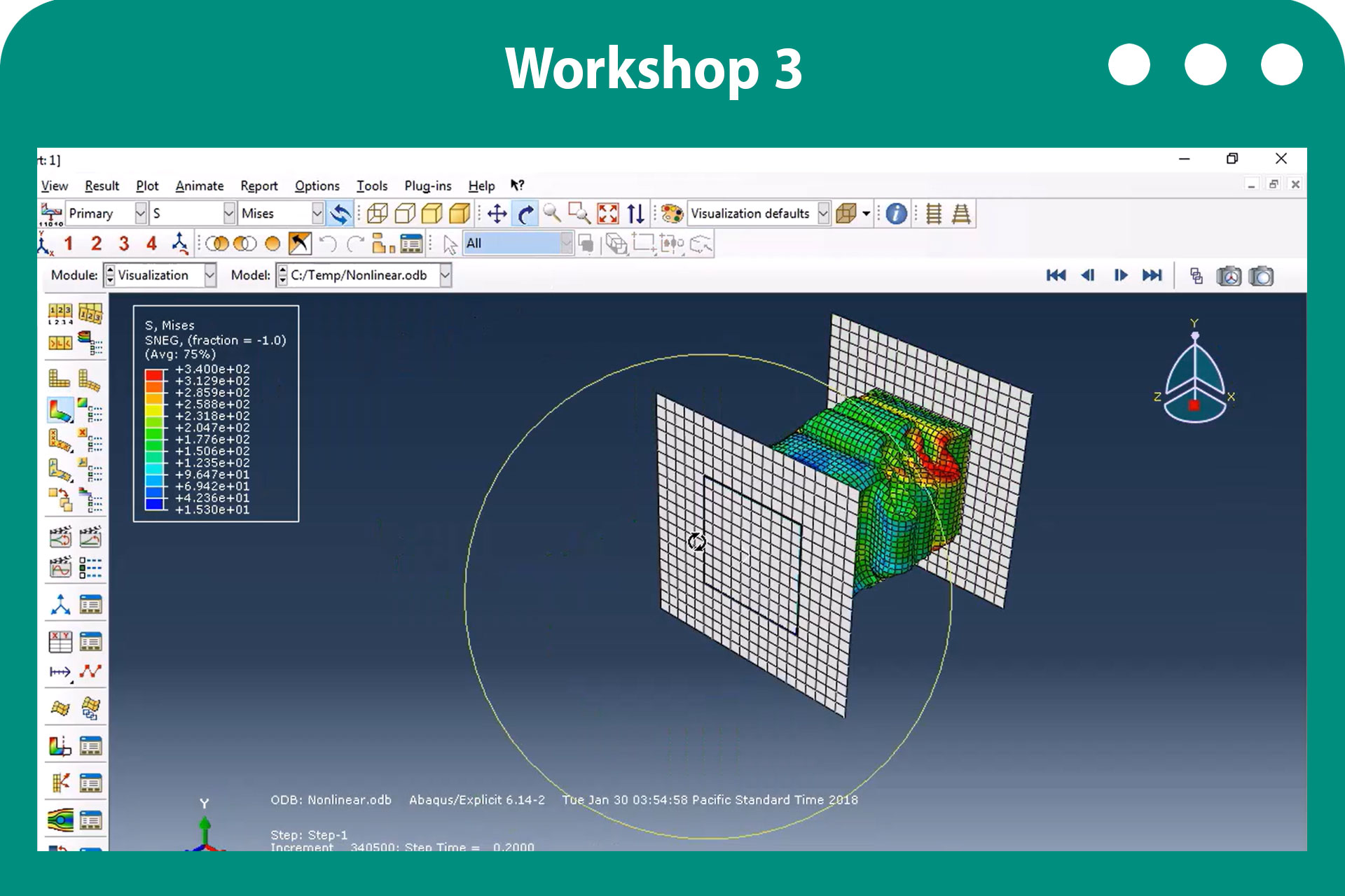
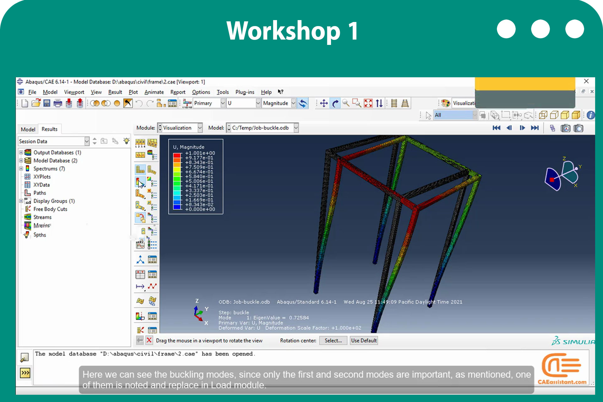
There are couple of examples to show you how to do nonlinear buckling in Abaqus in our Abaqus buckling tutorial: Workshops 1, 3, and 5.
8. Step by step example for Nonlinear Buckling in Abaqus
Now, it is time for practice. Let’s do the nonlinear buckling for the shell column which we did its linear buckling.
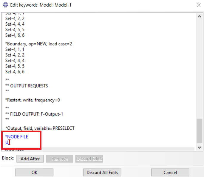
The modeling is the same but before we run the linear buckling, we must add a command to its input file. This command saves the model’s node file which will be used in the nonlinear buckling when we input the imperfection (see figure below).
Figure 16: Importing the node file command in the Buckle step
For nonlinear buckling, you don’t need to repeat all the steps to make the model; just create copy of the current model and make a few changes according to the following.
The changes needed for the new model to perform nonlinear buckling analysis are limited to adjustments in the Step and Load modules. Additionally, modifications in the model’s input file are required to include imperfections, which are essential for conducting nonlinear buckling analysis.
Step Module:
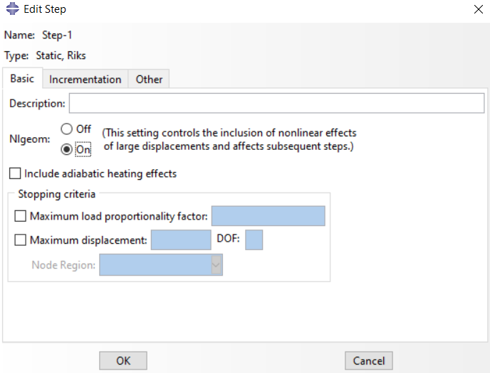
Go to the Step module and change the Step type to “Static, Riks” (fig 17). Enable the nonlinear option and accept other settings as default.
Figure 17: Choosing Static, Riks Step
Load Module:
In the Load module, due to the change in analysis type, check if the loading conditions have been removed. If so, reapply the load to the model. Next, it’s time to introduce imperfections to the model.
Adding Imperfection and run the Analysis:
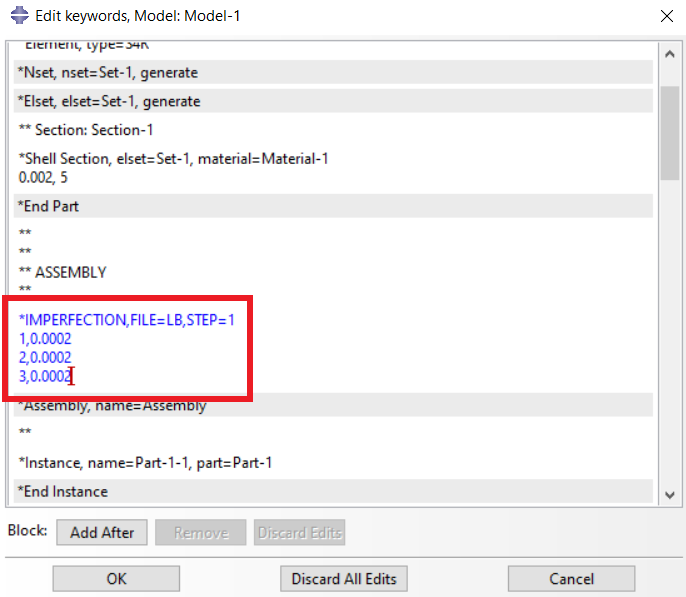
To do this, open the model’s input command file and enter the required command (see Figure 18). The filename in the command represents the Job name from the linear buckling analysis, and the Step specifies which step of the analysis the command should be applied to. In the following three lines, you define the magnitude of the imperfections. If the Node File command (fig 16) wasn’t used during the linear analysis, the run will result in an error.
Typically, the magnitude of the imperfections is about one-tenth of the shell’s thickness.
Figure 18: Adding Imperfection commands in input file
Now, all set and you just have to run the analysis and see the results.
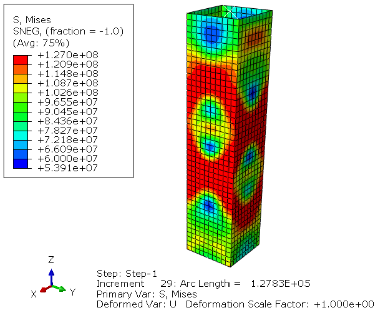
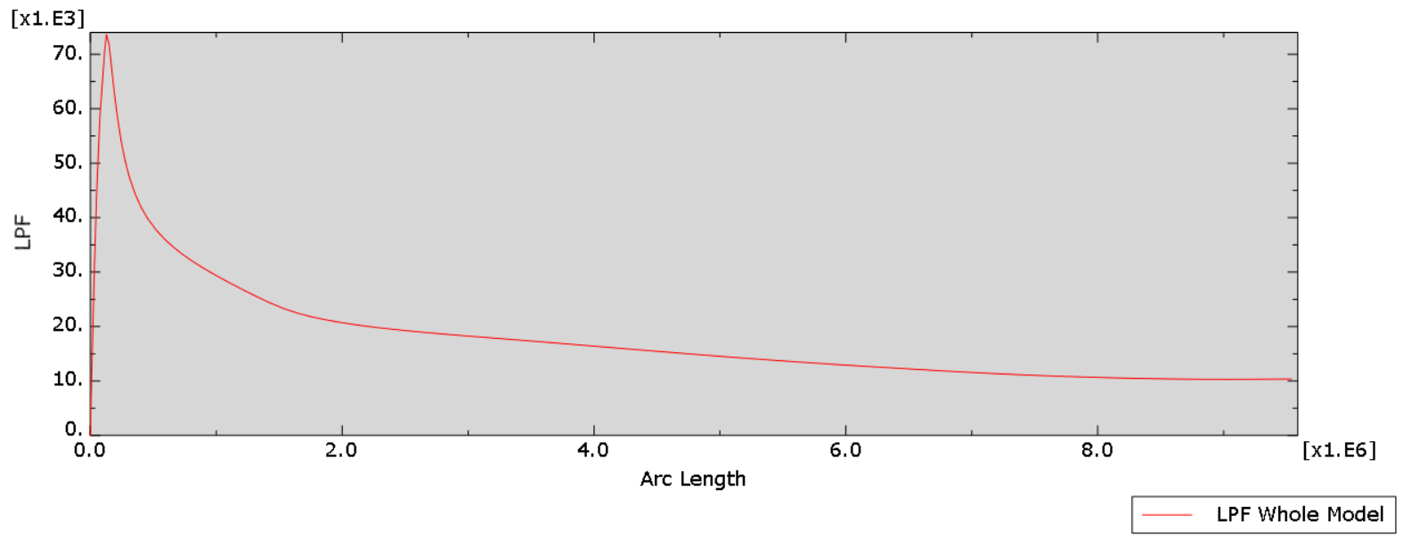
In figure 19 you can see when the column buckles and the critical buckling load would be approximately 73.6 KN according to the LPF (Load Proportionally Factor) diagram (fig 20). If you look at the figure 13 again (first eigenvalue in the linear buckling), you can see that the estimated buckling load in linear buckling is 80.8 KN; but now the critical buckling load in nonlinear buckling is 73.6 KN.
The results depend on mesh convergence and most of all the imperfections we enter. This was just an example to get more accurate results, we need to do mesh convergence and obtain the imperfection data from experimental data or any other methods.
Figure 19: Buckling stage
Figure 20: LPF diagram
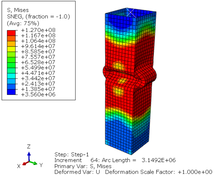
In the figure 21, you can see the postbuckling behavior of the model.
Figure 21: Postbuckling behavior
We have a tutorial video of the postbuckloing behavior of a frame in this lesson of our beginner package.
8.1. What is Load Proportionally Factor (LPF) diagram?
The Load Proportionality Factor (LPF) is a key result in the Riks method, representing how much the reference load is scaled during the analysis. It provides a direct measure of how the applied load progresses as the structure deforms. When combined with displacement data, the LPF forms a load-displacement curve, which is essential for understanding two critical aspects of buckling behavior: the critical buckling load (the peak of the curve) and the postbuckling behavior (how the structure responds after the peak, either stabilizing or collapsing).
The LPF diagram is this load-displacement curve, plotted to show how the structure’s load capacity evolves with increasing displacement. The horizontal axis represents the displacement at a critical point on the structure (e.g., the top of a column or center of a plate), indicating how much the structure deforms. The vertical axis represents the LPF (𝜆), which scales the reference load. By multiplying the LPF by the reference load, you can calculate the total load at any stage of the analysis.
The diagram has several key features:
- The peak point marks the critical buckling load, where the structure first becomes unstable.
- The descending branch shows postbuckling behavior, indicating whether the structure stabilizes (plateaus) or collapses (further descent).
- Before the peak, the structure is stable and can resist increasing loads; after the peak, its stiffness reduces, and instability occurs.
To interpret the results in Abaqus, you can extract LPF values directly from the output and use the load-displacement curve (fig 20). The maximum LPF indicates the critical buckling load, calculated as:
Where is the reference load (the one you input in the Load module). This curve also helps assess the structure’s behavior after buckling, providing insights into its safety and stability.
9. Conclusion
|
You can learn Abaqus from the very beginning with the package below: |
All about buckling analysis, practical examples to learn the buckling error-free in Abaqus. |
Explore our comprehensive Abaqus tutorial page, featuring free PDF guides and detailed videos for all skill levels. Discover both free and premium packages, along with essential information to master Abaqus efficiently. Start your journey with our Abaqus tutorial now!
The CAE Assistant is committed to addressing all your CAE needs, and your feedback greatly assists us in achieving this goal. If you have any questions or encounter complications, please feel free to share it with us through our social media accounts including WhatsApp.


