
Artificial Neural Networks for Short Fiber Composite Model

Short Fiber Reinforced Composites (SFRCs) are increasingly popular due to their suitability for injection molding and superior properties compared to unfilled polymers. Understanding their behavior is essential for predicting potential damage and optimizing their use in various applications.
To model SFRCs, we explore micro-mechanical approaches, focusing on mean-field and full-field models. While mean-field models are computationally efficient, they lack detailed insights. Full-field methods, though accurate, are time-intensive and require significant computational resources.
In this blog, we introduce the advantages of using neural networks for short fiber composite model over traditional methods for modeling SFRCs. We cover essential aspects like hidden layers, activation functions, training, validation, normalization, and evaluation. By the end, you will understand how to design and implement neural networks for accurate SFRC modeling and learn about the benefits and process of using these advanced techniques.
Understanding short fiber composites—and especially simulating their damage—can be tricky without the right guidance. That’s why we’ve created two tutorial packages!! Both packages aim to simulate damage in short fiber composites using Abaqus, they differ in their modeling approaches—macroscopic phenomenological modeling versus micromechanical homogenization—and the specific subroutines used for implementation.
|
This tutorial starts from the ground up, making it perfect if you’re new to short fiber composites. It explains the basics, focuses on simulating damage in short fiber composites using Dano’s macroscopic damage model. It provides detailed guidance on implementing the model in Abaqus through the VUSDFLD subroutine |
This package introduces a micromechanical approach to modeling short fiber composite damage using mean-field homogenization (MFH). It teaches how to implement this technique in Abaqus via a UMAT subroutine, offering a simplified method for analyzing the material’s stiffness and strength based on fiber and matrix properties. |

1. Short Fiber Composite and Micro-Mechanical Modeling Approaches
Short Fiber Reinforced Composites (SFRCs) have become increasingly popular in various applications, primarily because they are well-suited for injection molding techniques and offer enhanced properties compared to unfilled polymers. Consequently, it is crucial to model the behavior of these short-fiber composites to anticipate potential damage.
To model the behavior of short fiber composites in a general way Micro-mechanical modeling approaches These models can be generally categorized into two major classes: mean-field and full-field models.
Mean-field models take into account average stress and strain within the microstructural components, making them computationally efficient. However, these models do not provide detailed insights into the deformation mechanisms at the microstructural level or the interactions between different phases. Additionally, they lack the accuracy of full-field models.
Traditional full-field methods utilize detailed and thorough simulations to accurately represent the behavior of materials or systems throughout the entire area of interest. These methods often involve creating an appropriate Representative Volume Element (RVE) through a trial-and-error approach. This approach is both computationally demanding and time-intensive, as it requires simulating the material’s behavior under different conditions to ensure precision. Additionally, traditional full-field methods consume considerable amounts of memory and computational power to maintain and analyze the extensive data needed for precise modeling.
Using a neural network for modeling has several advantages over traditional full-field methods:
2. A micromechanics-based artificial neural network
Input Parameters: Neural networks use the orientation tensor and volume fraction as inputs, allowing for modeling with desired properties and full-field level accuracy without the trial-and-error process of generating a proper RVE realization.
Memory and Computational Time: Neural networks use weights and biases to store learned knowledge, significantly reducing the amount of memory and computational time needed.
Transfer Learning: Neural networks can utilize transfer learning to enhance models. For example, a neural network can inherit normalization and trainable parameters from an original network and be fine-tuned with a new data set, improving accuracy with less data.
Handling Unseen Conditions: Fine-tuned neural networks, which are first trained on a larger data set and then fine-tuned with a smaller one, can handle unseen loading conditions with highly accurate predictions.
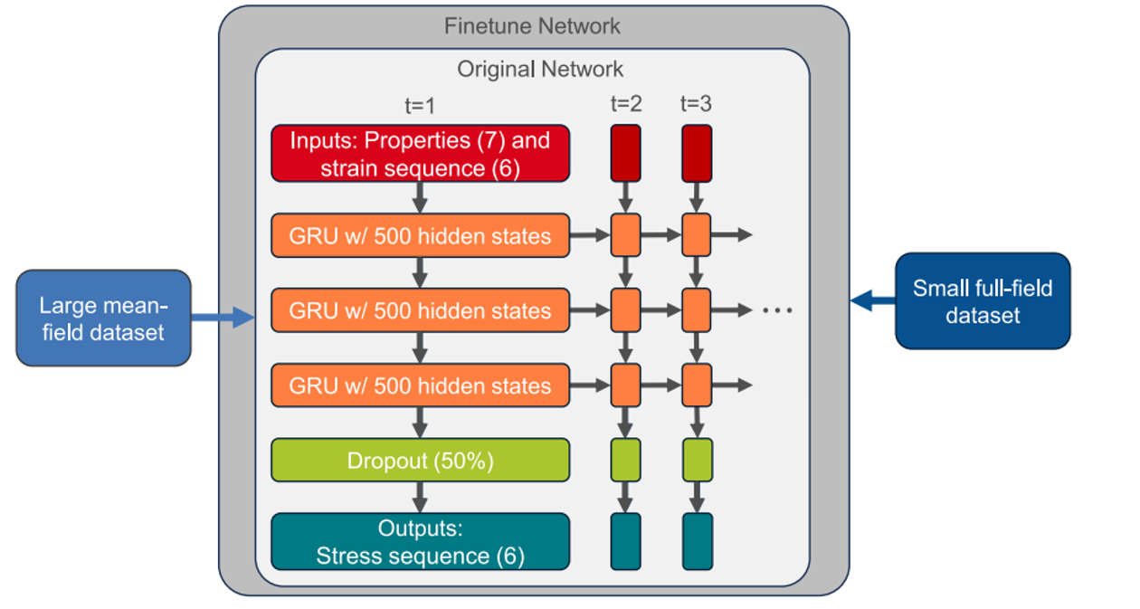
Figure 1: Network architecture and the transfer learning approach utilizing a large mean-field and a small full-field data set
3. How the neural network is modeled?
In neural network modeling, key elements include hidden layers, activation functions, training, validation, normalization, and evaluation. Dense hidden layers enable the network to approximate intricate functions by fully connecting neurons across layers. The Exponential Linear Unit (ELU) activation function introduces non-linearity, enhancing the network’s ability to learn complex patterns. Training involves iterative weight adjustments to minimize loss, while validation evaluates the model’s performance on unseen data to detect overfitting. Normalizing input data to a common range, typically [0, 1], promotes efficient learning and quicker Abaqus convergence. Evaluation employs metrics like Mean Relative Error (MeRE) and Maximum Relative Error (MaRE) to thoroughly assess model performance, ensuring the neural network is robust, accurate, and adept at handling complex data patterns.
In modeling a neural network, key components such as hidden layers, activation functions, training, validation, normalization, and evaluation are essential. The hidden layers, specifically dense layers, enable the neural network to approximate complex mathematical functions by connecting each neuron in one layer to every neuron in the previous layer. The Exponential Linear Unit (ELU) activation function introduces non-linearity, enhancing the network’s ability to learn intricate patterns.
Training involves adjusting weights over multiple epochs to minimize the loss function, while validation assesses the model’s generalization ability on unseen data, aiding in overfitting detection. Normalization of input data to a common range, typically [0, 1], ensures efficient learning and faster convergence. Finally, the evaluation process uses metrics like Mean Relative Error (MeRE) and Maximum Relative Error (MaRE) to provide a comprehensive assessment of the model’s performance. This holistic approach ensures that the neural network is robust, accurate, and capable of handling complex data patterns.
Now, let’s explain each one in detail.
3.1. Design of Hidden Layers
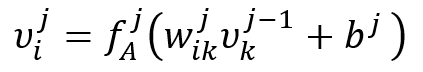
The hidden layers in the neural network can approximate any mathematical functions. In this study, only dense layers are used. In dense layers, each neuron in one layer is connected to all neurons in the previous layer. In the design of hidden layers within a neural network, dense layers are a common and fundamental component. A dense layer, also known as a fully connected layer, is one where each neuron in the layer is connected to every neuron in the previous layer. This means that the value of a neuron ![]() in one layer is linked to all neurons
in one layer is linked to all neurons ![]() of the previous layer.
of the previous layer.
The calculation of ![]() is performed using an activation function
is performed using an activation function ![]() with weights
with weights ![]() and biases
and biases ![]() as follows:
as follows:
In this setup:
![]() is the value of the neuron in the current layer.
is the value of the neuron in the current layer.
![]() are the values of the neurons in the previous layer.
are the values of the neurons in the previous layer.
![]() are the weights associated with the connections between neurons.
are the weights associated with the connections between neurons.
![]() are the biases for the neurons.
are the biases for the neurons.
![]() is the activation function applied to the weighted sum of inputs plus the bias.
is the activation function applied to the weighted sum of inputs plus the bias.
Dense layers are used to approximate any mathematical function and are essential for the neural network’s ability to learn complex patterns in the data. They are particularly useful in scenarios where the relationships between input and output data are intricate and require a high level of connectivity to capture effectively.
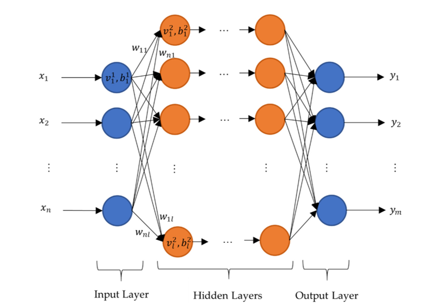
Figure2: Schematic design of neural network with dense layers
3.2. An activation function
An activation function in a neural network is a mathematical function applied to the output of a neuron. It determines whether a neuron should be activated or not, essentially deciding if the neuron’s input to the network is relevant for the prediction process. Activation functions introduce non-linearity into the network, enabling it to learn and model complex data patterns. Here are some key points about activation functions based on the provided snippets:
Elu (Exponential Linear Unit):
The Exponential Linear Unit (ELU) is an activation function used in neural networks to introduce non-linearity, which helps the network learn complex patterns in the data. The ELU activation function is defined as:
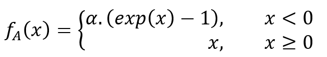
Here a denotes a scalar and x the input of a neuron. ![]() a scalar that determines the value to which an ELU saturates for negative net inputs. It is a hyperparameter that can be tuned. ELU is used for all hidden layers in the work described in the snippets. ELU can lead to faster convergence during training compared to other activation functions like ReLU.
a scalar that determines the value to which an ELU saturates for negative net inputs. It is a hyperparameter that can be tuned. ELU is used for all hidden layers in the work described in the snippets. ELU can lead to faster convergence during training compared to other activation functions like ReLU.
3.3. Training and Validation
Training and validation are crucial steps in the development and evaluation of neural networks. Training is the process where the neural network learns from the data. During training:
- Data Split: The dataset is divided into two parts: training data and validation data. In the study mentioned, the data is split in a ratio of ¾ for training and ¼ for validation.
- Weight Adjustment: The neural network adjusts its weights based on the training data to minimize the loss function, which measures the difference between the predicted and actual values.
- Epochs: The training process is carried out over multiple epochs, where an epoch is one complete pass through the entire training dataset.
- Loss Evaluation: The loss (or error) is calculated for the training data to monitor how well the network is learning.
Validation is the process of evaluating the neural network’s performance on a separate set of data that it has not seen during training. This helps in assessing the model’s ability to generalize to new, unseen data. During validation:
- Data Split: As mentioned, a portion of the data is set aside as validation data.
- No Weight Adjustment: The weights of the neural network are not adjusted based on the validation data. Instead, the validation data is used to evaluate the model’s performance.
- Validation Loss: The loss is calculated for the validation data to monitor how well the network is performing on unseen data. This helps in detecting overfitting.
- Overfitting Detection: Overfitting occurs when the neural network performs well on the training data but poorly on the validation data. By comparing the training loss and validation loss, overfitting can be detected and controlled.
3.4. Normalization
Normalization is a preprocessing step in machine learning and neural networks that involves scaling the input data to a specific range, typically [0, 1] or [-1, 1]. This process ensures that all input features contribute equally to the learning process and helps improve the convergence speed and performance of the model. Normalization ensures that different entries of the data, such as the stiffness tensor, are treated equally. Without normalization, features with larger ranges could dominate the learning process, leading to biased training. By scaling the data to a common range, the optimization algorithms used in training neural networks can converge faster and more efficiently. Normalization helps in avoiding numerical instability issues that can arise due to large variations in the input data.
Normalization typically involves scaling the data to a specific range. the output is normalized to the interval [0, 1]. The formula used for normalization is:
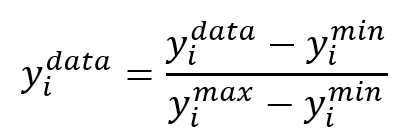
Where: ![]() is the normalized value of the data point.
is the normalized value of the data point. ![]() is the minimum value of the data point in the dataset.
is the minimum value of the data point in the dataset. ![]() is the maximum value of the data point in the dataset. By normalizing the data, the neural network can learn more effectively and produce better results.
is the maximum value of the data point in the dataset. By normalizing the data, the neural network can learn more effectively and produce better results.
3.5. Evaluation
Evaluation in the context of neural networks involves assessing the performance of the model to ensure it meets the desired criteria. Here are some key points from the provided information:
Loss Function: During training, the loss function is used to evaluate the network’s performance. However, it may not be ideal for reviewing performance across different test samples due to its lack of normalization.
Alternative Metrics: To address the limitations of the loss function, alternative metrics like the equivalent von Mises stress are used. This metric helps in determining the Mean Relative Error (MeRE) and Maximum Relative Error (MaRE), providing a more meaningful evaluation of the neural network’s performance. the evaluation process ensures that the neural network performs well not just on the training data but also on new, unseen data.
4. Use neural networks for short fiber composite model
In utilizing neural networks for short fiber composite model, the process begins with defining the composite structure through material selection, determining volume fractions, and defining geometry, material properties, boundary conditions, and loading scenarios. The composite’s fiber and matrix materials are chosen, and the fiber volume fraction is calculated to ensure accurate property prediction. The orientation of fibers and their probability distribution are modeled to represent the composite’s structural complexity accurately.
To capture the intricate relationships between input parameters and output properties, hidden layers in the neural network play a crucial role. During the pre-training phase, the network is exposed to extensive datasets, helping it learn general patterns and features. Fine-tuning follows with high-fidelity data from finite element method (FEM) simulations or experimental results to enhance model accuracy. This process ensures the network’s robust performance, capable of predicting mechanical properties effectively. The evaluation phase uses metrics like Mean Relative Error (MeRE) and Maximum Relative Error (MaRE) to compare the neural network’s predictions with actual composite behavior, highlighting the benefits of pre-training and fine-tuning in composite analysis.
Jumpstart your knowledge about short fiber composites: Introduction to short fiber composites, Advantages of short fiber composites, Application of short fiber composites, and short fiber composite modeling explained.

4.1. Modeling the Composite Structure
For each short fiber composite geometric structure, it will be done in the following order:
Material Selection:
Fiber and Matrix Selection: Choose the type of fibers (e.g., glass, carbon, aramid) and the matrix material (e.g., epoxy, polyester) that will be used in the composite.
Volume Fraction:
Determine the volume fraction of fibers and matrix. This ratio affects the overall properties of the composite. The fiber volume fraction (φ) is a measure of the amount of fiber present in a composite material relative to the total volume of the composite.
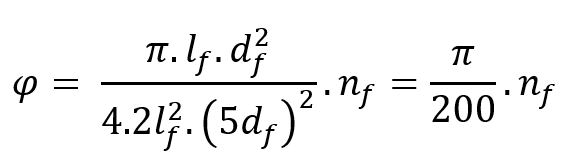
where ![]() and
and ![]() represent the length and diameter of fibers, and
represent the length and diameter of fibers, and ![]() is a positive integer number representing the number of fibers inside the RVE. Using this approach for the RVE size, it is not possible to obtain a continuous field of fiber volume fraction because it relies on the discrete field of the number of fibers. Therefore, a modification is introduced with a scaling factor a:
is a positive integer number representing the number of fibers inside the RVE. Using this approach for the RVE size, it is not possible to obtain a continuous field of fiber volume fraction because it relies on the discrete field of the number of fibers. Therefore, a modification is introduced with a scaling factor a: ![]() ,
, ![]() . Consequently,
. Consequently, ![]() becomes dependent on
becomes dependent on ![]() , allowing for the acquisition of continuous values of fiber volume fractions.
, allowing for the acquisition of continuous values of fiber volume fractions.
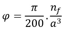
the scaling factor should be greater than or equal to one to maintain the minimum RVE dimensions ![]() . By increasing the scaling factor from one, different fiber volume fractions can be obtained for a specific number of fibers. To avoid large scaling factors and thus large RVEs and high computational costs, different numbers of fibers and their corresponding scaling factors are selected for different ranges of fiber volume fraction.
. By increasing the scaling factor from one, different fiber volume fractions can be obtained for a specific number of fibers. To avoid large scaling factors and thus large RVEs and high computational costs, different numbers of fibers and their corresponding scaling factors are selected for different ranges of fiber volume fraction.
Geometry Definition:
Shape and Size: Define the overall shape and size of the composite structure. This could be a plate, beam, shell, or any other structural form. In short fibers, fiber orientation is very important. The fiber orientation is represented by a unit vector ![]() , which can be described by two angles
, which can be described by two angles ![]() and
and ![]() . The orientation vector
. The orientation vector ![]() in Cartesian coordinates is given by:
in Cartesian coordinates is given by:
![]()
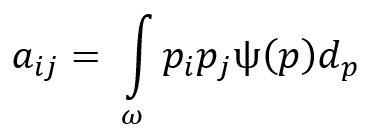
To describe the fiber orientation distribution at a material point, a probability distribution function p is needed. Using the orientation distributions and the probability distribution function, a second-order tensor can be defined to describe the orientation distribution. The components of this tensor are given by:
Orientation distributions are generated by creating diagonal orientation tensors for different cases: in 3D random distribution ![]() , Planar random distribution
, Planar random distribution ![]() .
.
Material Properties:
Elastic Properties: Assign the elastic properties to each layer, including: Young’s Modulus (E): Measure of stiffness in the fiber direction (![]() ) and transverse direction (
) and transverse direction (![]() ) Shear Modulus (G): Measure of the material’s response to shear stress. Poisson’s Ratio (ν): Ratio of transverse strain to axial strain. Strength Properties: Define the tensile, compressive, and shear strengths of the material. Thermal Properties: If the analysis involves thermal effects, include properties like thermal expansion coefficients and thermal conductivity.
) Shear Modulus (G): Measure of the material’s response to shear stress. Poisson’s Ratio (ν): Ratio of transverse strain to axial strain. Strength Properties: Define the tensile, compressive, and shear strengths of the material. Thermal Properties: If the analysis involves thermal effects, include properties like thermal expansion coefficients and thermal conductivity.
Boundary Conditions and Loading:
Supports and Constraints: Define how the composite structure is supported. This could include fixed supports, simply supported edges, or free edges.
Loading Conditions: Specify the types of loads the structure will experience, such as tensile, compressive, bending, or shear loads. Include the magnitude and direction of these loads.
Meshing:
Element Type: Choose the type of finite elements to be used (e.g., shell elements for thin structures, solid elements for thick structures).
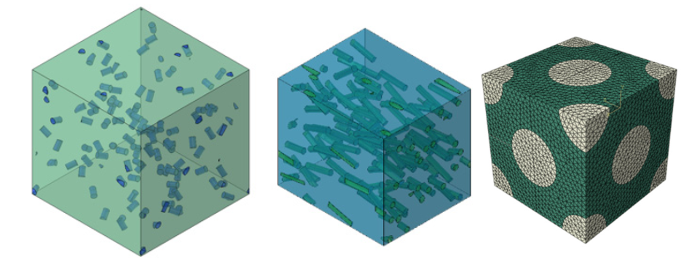
Figure 3: Meshing of RVE
4.2. Model Selection
In order to utilize artificial intelligence for damage assessment, it is essential to establish the damage model. This model can be derived from various approaches, such as the Hashin Damage criteria, the Lemaitre model, or a pseudo-grain failure model employing conventional models as references.
The pseudo-grain failure model aims to simulate the progressive failure of composites by considering the misalignment of short fibers within the matrix. This is particularly useful for short fiber thermoplastics. The model divides the composite material into pseudo-grains, each representing a small volume of the composite with a specific fiber orientation. It accounts for the inelastic behavior of the composite by modeling the damage and failure of these pseudo-grains under various loading conditions.
The difference between two short fiber composite damage tutorial packages in modeling:
- Damage simulation of short fibre composites with subroutine: Utilizes a macroscopic damage model (Dano’s model) implemented via the VUSDFLD subroutine.
- Short fiber composite damage (Mean Field Homogenization Model): Employs a micromechanical approach using mean-field homogenization implemented through a UMAT subroutine.
4.3. Data Collection for obtaining damage response in Artificial Neural Model damage
Collect experimental data to validate the model. This can include measurements of Young’s moduli, fracture toughness, and other mechanical properties. Use simulation tools like Digimat-MF to perform mean-field homogenization and predict the mechanical properties of the composite. These tools can help in comparing the model predictions with experimental results.
4.4. Hidden layer in composite
For modeling composites using a neural network, the hidden layers are crucial in capturing the complex relationships between input parameters and the desired output properties. hey are the computational workhorse of deep learning models, allowing neural networks to approximate functions and capture patterns from input data collection.
Pre-training and Hidden Layers:
During the pre-training phase, the neural network, including its hidden layers, is trained on a large dataset (e.g., homogenization data). This helps the network, particularly the hidden layers, to learn general features and patterns in the data. The hidden layers capture these learned features, which form the basis for further fine-tuning.
Hidden layers in a neural network are responsible for extracting features from the input data. During pre-training, these layers learn to identify and represent important patterns and structures in the data. Pre-training helps in initializing the weights of the hidden layers in a way that they are already tuned to capture general features. This makes the subsequent fine-tuning phase more effective and faster. In a typical neural network training process, weights are often initialized randomly. This can sometimes lead to poor convergence or getting stuck in local minima. With weights initialized through pre-training, the network is already somewhat aligned with the underlying data distribution. This makes the fine-tuning phase more efficient, as the network requires fewer adjustments to reach optimal performance. By starting with pre-trained weights, the network is less likely to overfit the smaller, task-specific dataset during fine-tuning. This is because the initial weights already encode general knowledge, reducing the risk of the network becoming too specialized to the fine-tuning data.
Pre-training on a large dataset helps the hidden layers to generalize well, meaning they can capture features that are not specific to the training data but are applicable to a broader range of data.
– This generalization is essential for the transfer learning process, as it allows the pre-trained model to serve as a good starting point for fine-tuning on more specific datasets.
Fine-tuning with FEM or Experimental Data (Fine-tuning Phase:):
The pre-trained model is then fine-tuned using a smaller, more precise dataset obtained from FEM simulations or experimental data. This step enhances the model’s accuracy and performance. A smaller but high-fidelity dataset is generated using FEM simulations.
The pre-trained model, which has been trained on a large dataset (mean-field data set), is used as the starting point. The fine-tuning is performed using a smaller, high-fidelity dataset (full-field data set). The fine-tuning involves adjusting all trainable parameters of the pre-trained model using the high-fidelity data. This approach consistently yields better performance compared to partial fine-tuning (freezing some parameters).
This detailed process highlights the importance of using a pre-trained model and fine-tuning it with high-fidelity data to achieve better performance and accuracy in predictions.
- Performance Comparison (Evaluation in composite):
The performance of the transfer learning model is compared with a model trained solely on the high-fidelity dataset. One of these methods is mean relative error (MeRE) and maximum relative error (MaRE) . The Mean Relative Error (MeRE) and Maximum Relative Error (MaRE) are key metrics used to evaluate the performance of neural networks in predicting the properties of short fiber reinforced composites.
Understanding short fiber composites—and especially simulating their damage—can be tricky without the right guidance. That’s why we’ve created two tutorial packages!! Both packages aim to simulate damage in short fiber composites using Abaqus, they differ in their modeling approaches—macroscopic phenomenological modeling versus micromechanical homogenization—and the specific subroutines used for implementation.
|
This tutorial starts from the ground up, making it perfect if you’re new to short fiber composites. It explains the basics, focuses on simulating damage in short fiber composites using Dano’s macroscopic damage model. It provides detailed guidance on implementing the model in Abaqus through the VUSDFLD subroutine |
This package introduces a micromechanical approach to modeling short fiber composite damage using mean-field homogenization (MFH). It teaches how to implement this technique in Abaqus via a UMAT subroutine, offering a simplified method for analyzing the material’s stiffness and strength based on fiber and matrix properties. |
The CAE Assistant is committed to addressing all your CAE needs, and your feedback greatly assists us in achieving this goal. If you have any questions or encounter complications, please feel free to share it with us through our social media accounts including WhatsApp.
5. Conclusion
In the end Short Fiber Reinforced Composites (SFRCs) are favored for injection molding due to their enhanced properties compared to unfilled polymers. Two main micro-mechanical modeling approaches, mean-field and full-field models, are used to predict damage. Mean-field models, which average stress and strain within microstructural components, offer computational efficiency but lack detailed insights into deformation mechanisms and phase interactions, leading to lower accuracy than full-field models. Full-field models, which simulate material behavior in detail, require significant computational resources for creating and analyzing Representative Volume Elements (RVE). Neural networks provide a superior alternative, achieving desired properties and full-field level accuracy without the trial-and-error process of generating an RVE. They use weights and biases to store learned knowledge, reducing memory and computational time, and can leverage transfer learning to enhance models with less data. Fine-tuned neural networks for short fiber composite model can predict unseen loading conditions with high accuracy.
Key elements in neural network modeling include hidden layers, activation functions, training, validation, normalization, and evaluation. Dense hidden layers approximate complex functions, while the ELU activation function introduces non-linearity to enhance pattern learning. Training involves iterative weight adjustments to minimize loss, and validation assesses the model’s generalization on unseen data to detect overfitting. Normalization scales input data to a common range (typically [0, 1]) for efficient learning and faster convergence. Evaluation metrics like Mean Relative Error (MeRE) and Maximum Relative Error (MaRE) provide a thorough assessment of model performance. In composite modeling, crucial steps include material selection, volume fraction determination, geometry definition, and material property assignment. Boundary conditions and loading scenarios are defined, and meshing involves selecting appropriate finite elements. The process includes pre-training the neural network on extensive datasets for general pattern learning and fine-tuning with high-fidelity data from FEM simulations or experiments, ensuring robust and accurate predictions.