In-depth overview of Abaqus Crack and Fracture Mechanics: Principals, Applications, and Methods

Did you know that tiny cracks in materials can lead to sudden failures in structures, even under normal loads? Understanding how these cracks form and grow is critical for designing safe and durable systems.

Fracture mechanics is the science that studies the behavior of materials with cracks under stress. By analyzing factors such as crack initiation and growth, engineers can predict failures and develop effective solutions to prevent them. Advanced simulation tools like Abaqus—with its robust Abaqus Crack capabilities—enable precise modeling of these processes, making it an invaluable resource for both engineers and researchers.

In this blog, we explore the principles of fracture mechanics and how Abaqus is used to simulate crack behavior. You will learn about methods like Griffith’s theory, fracture modes, and advanced tools such as XFEM and cohesive zone modeling. The blog also discusses practical applications, from fatigue crack analysis to machine learning integration, providing a comprehensive guide for anyone interested in this field.

Are you looking to master fracture mechanics and crack modeling in Abaqus? Our comprehensive tutorials offer step-by-step guidance on simulating crack propagation across various materials, including concrete, steel, and bone. With over 300 minutes of detailed video content, these tutorials cover essential methods such as XFEM, J-integral, and H-integral. Also, there are 2D and 3D crack propagation simulation in our tutorial videos.

1. What is Fracture Mechanics and Why is it Important? Abaqus Fracture analysis

Fracture mechanics is the study of how materials with cracks behave under stress, focusing on understanding the processes behind crack initiation, growth, and propagation. This field plays a crucial role in predicting and preventing failures in structures, thereby enabling the design of safer and more resilient materials. By examining factors such as the material’s structure, the type of force applied, and environmental conditions, fracture mechanics distinguishes between behaviors like brittle failure—where materials break suddenly with little deformation—and ductile failure, where materials absorb energy and deform before fracturing. Understanding these key concepts, including fracture, crack, and failure, is essential for effective analysis and design in engineering.

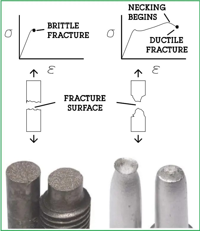
Figure 1: Demonstrates how brittle and ductile fractures occur in materials

2. Fundamentals of Fracture Analysis

In this section, we’ll dive into Griffith’s Theory of Crack Propagation and explore how cracks develop and spread in brittle materials. We’ll also look into two primary approaches in fracture mechanics—Linear Elastic Fracture Mechanics (LEFM) and Elastic-Plastic Fracture Mechanics (EPFM)—and the different modes of fracture that can occur. By understanding these concepts, you’ll get a better idea of how cracks behave and how we can predict and prevent failures in materials. Let’s break it down step by step!

Fracture mechanics can be classified into two main categories based on the material behavior:

In summary, LEFM and EPFM are two distinct approaches in fracture mechanics. LEFM assumes a linear elastic response at the crack tip—ideal for brittle materials—where deformations are reversible. In contrast, EPFM incorporates elastic-plastic behavior, accounting for non-linear and irreversible deformations typical of ductile materials.

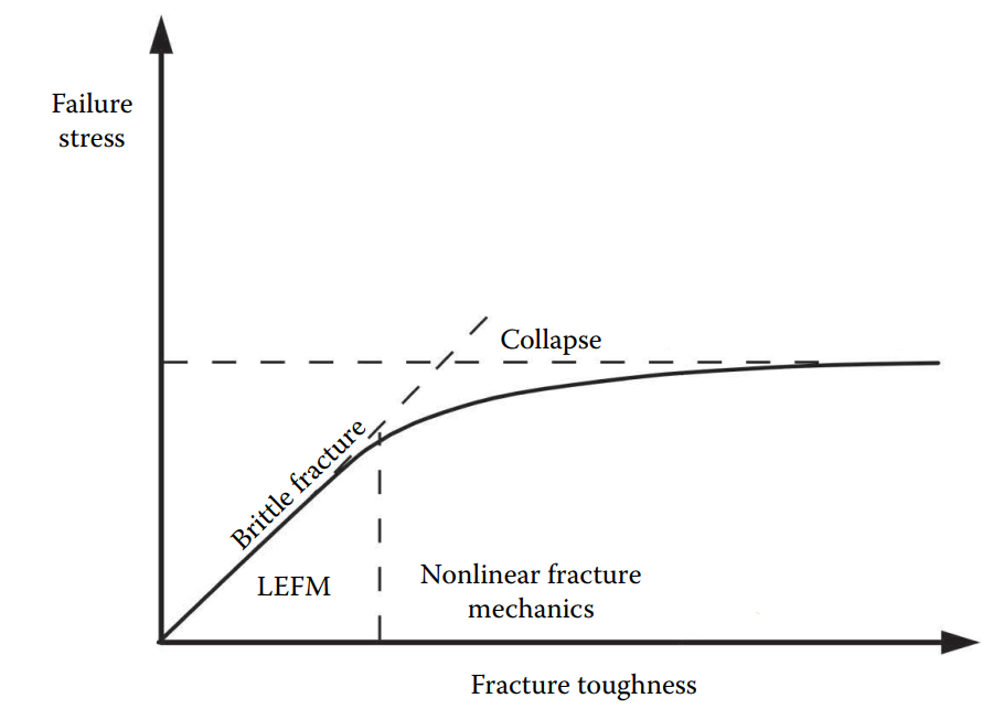
Figure 2: LEFM VS EPFM

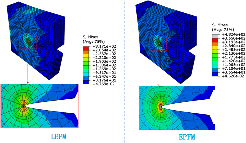
Figure 3: Deformation comparison between LEFM and EPFM [Ref]

2.3. Fracture Analysis Methods

Fracture analysis methods are used to analyze the behavior of materials under loading and to predict the critical stress or displacement required for crack initiation and growth. Linear Elastic Fracture Mechanics (LEFM) methods assume linear elastic behavior near the crack tip, while Elastic-Plastic Fracture Mechanics (EPFM) methods account for elastic-plastic behavior. LEFM methods typically involve calculating the stress intensity factor (SIF) or the strain energy release rate at the crack tip, while EPFM methods involve calculating the J-integral or the crack tip opening displacement (CTOD) using plastic zone size correction factors. Other fracture analysis methods include cohesive zone modeling, continuum damage mechanics (CDM), and fracture toughness testing. Some of the mentioned methods could be used in both LEFM and EPFM but with their proper modifications.

In the following, the most important methods will be sufficiently explained.

2.3.1. Stress Intensity Factor (SIF)

The stress intensity factor (SIF) method is a fundamental concept in fracture mechanics that is used to predict the behavior of materials near the crack tip. It is based on the assumption that the material behavior near the crack tip is linearly elastic, which is valid for brittle materials such as ceramics and glasses. The SIF method can be applied to a wide range of geometries, including cracks in plates, shells, and beams. Analytical solutions are available for simple geometries, while numerical techniques, such as the finite element method, are used for more complex geometries.

2.3.2. Energy approach

The energy method involves analyzing the energy balance between the energy required to create new surfaces due to crack propagation and the energy released by the stresses around the crack tip. It is a general approach that can be applied to both brittle and ductile materials.

The energy Griffith method: The energy Griffith method is a specific application of the energy method developed by A.A. Griffith to predict the critical stress required for crack propagation in brittle materials.

2.3.3. J-Integral

The J-integral is a mathematical concept used in fracture mechanics to quantify the amount of energy required to create new crack surfaces and to deform the material near the crack tip. It is a key concept in Elastic-Plastic Fracture Mechanics (EPFM) and is used to account for the plastic deformation that occurs near the crack tip.

The J-integral method is particularly useful for analyzing the behavior of ductile materials, such as metals, where significant plastic deformation occurs near the crack tip. It can be used to predict the critical stress required for crack initiation and growth under both monotonic and cyclic loading conditions.

2.3.4. Fracture toughness

Fracture toughness is a fundamental material property in fracture mechanics that describes the ability of a material to resist the propagation of a crack. It is a measure of the material’s resistance to fracture when subjected to a high-stress load.

Fracture toughness is typically defined as the critical stress intensity factor (Kc) required to propagate a crack in a material. It represents the resistance of the material to the growth of an existing crack and is a key parameter in the design and analysis of structural components.

2.3.5. Crack Tip Opening Displacement (CTOD)

The Crack Tip Opening Displacement (CTOD) method is a measure of the amount of displacement or opening that occurs at the tip of a crack when a load is applied. The CTOD method is particularly useful for analyzing the behavior of ductile materials, such as metals, where significant plastic deformation occurs near the crack tip. It can be used to predict the critical stress required for crack initiation and growth under both monotonic and cyclic loading conditions.

2.3.6. R-curve

The R-curve is a fracture mechanics concept that describes the relationship between the crack growth resistance and the crack extension in a material. It is a measure of the material’s ability to resist crack propagation as the crack grows and is commonly used in Elastic-Plastic Fracture Mechanics (EPFM).

The R-curve is obtained by plotting the crack extension (δa) against the crack growth resistance (R) for a given material. The crack growth resistance is typically defined as the slope of the load-displacement (P-δ) curve, which represents the energy required to propagate the crack.

2.4. Griffith’s Theory of Crack Propagation

Griffith’s theory is a fascinating way to understand how cracks begin and spread in brittle materials. Developed by Alan Griffith in 1920, this concept explains that tiny cracks or imperfections can significantly weaken a material. These little flaws act as stress hotspots, and how they respond can determine if the material will hold up or eventually break.

When a crack forms and begins to grow in a brittle material, it releases elastic strain energy, which drives the crack to spread further. At the same time, creating new surfaces as the crack expands requires energy, known as surface energy. According to Griffith’s criterion, a crack will continue to grow if the strain energy release rate (G) equals or exceeds the energy needed to form new crack surfaces (2γ, where γ is the surface energy per unit area).

For example, consider a large brittle plate with a single central crack of length 2a, as shown in Fig. 2. When a uniform tensile load is applied perpendicular to the crack plane along the x-axis, the material releases elastic strain energy stored within a cylindrical volume of length B. This released energy is calculated as the product of the strain energy density (R_d) and the cylindrical volume surrounding the crack (2πa²B). If this released energy is sufficient to overcome the surface energy required to create new crack surfaces, the crack will continue to propagate.

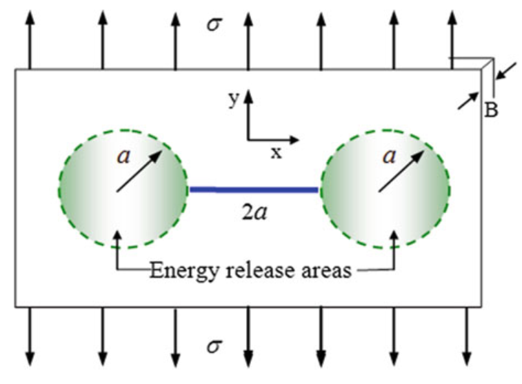
Figure 4: A large plate containing one through-thickness central crack. Also shown are two idealized energy-release areas ahead of the crack tips

The strain energy release rate, 𝐺 depends on the material’s properties, the applied stress (𝜎), and the crack size (𝑎). For a simple case of a centrally located crack in an infinite plate under uniform tensile stress, 𝐺 can be calculated using:

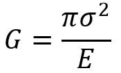
Here, E is the material’s modulus of elasticity. In finite element analysis, particularly with software like Abaqus, the parameters related to stress and strain energy release are applied as model inputs and boundary conditions to study the material behavior around cracks under stress. This analysis helps determine whether a crack will propagate spontaneously or not. By using finite element analysis in Abaqus, the precise effects of cracks on the overall material performance and their propagation behavior can be simulated, providing accurate predictions of material failure under real-world conditions.

2.5. What are the three Fracture Modes?

The term “fracture modes” describes the way crack tip stresses are separated into three different types of loads, also known as “modes”. There are three fracture modes:

1. Mode I fracture: Also known as opening mode or tensile mode fracture. In this mode, the crack surfaces are pulled apart, causing the crack to open perpendicular to the direction of the applied load. Mode I fracture is often associated with ductile materials such as metals and polymers.
2. Mode II fracture: Also known as sliding mode or in-plane shear mode fracture. In this mode, the crack surfaces slide past each other in a direction parallel to the direction of the applied load. Mode II fracture is often associated with materials that are strong in shear, such as composites.
3. Mode III fracture: Also known as tearing mode or out-of-plane shear mode fracture. In this mode, the crack surfaces move in opposite directions parallel to the direction of the applied load. Mode III fracture is often associated with materials that are brittle and have a low resistance to shear.

It is important to note that in reality, a fracture may involve a combination of these modes, depending on the material properties, loading conditions, and geometry of the structure. Nevertheless, grasping the modes of fracture is crucial for understanding “Abaqus Fracture Simulation,” predicting and preventing failures in materials and structures, and designing safer and more reliable structures capable of withstanding various loading conditions.

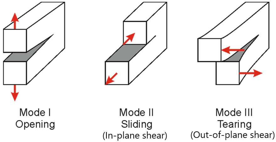
Figure 5: Three Fracture Modes [Ref]

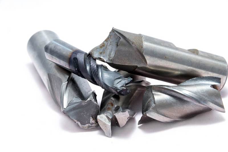
Figure 6: Fracture of drill bits

3. Fracture Simulation in Abaqus 

In this section, we’ll dive into why Abaqus is such a great tool for fracture mechanics analysis. From simulating crack initiation to predicting crack growth in materials, Abaqus offers powerful features like XFEM and Cohesive Zone Modeling that allow us to accurately analyze how materials behave under stress. You can learn the 2D and 3D XFEM simulation in Abaqus through our “Simulation fracture in Abaqus” tutorial.

We’ll also look at the initial steps required for crack analysis and how to simulate fatigue crack growth, particularly using the Paris-Erdogan law. Plus, we’ll explore a practical example of fracture analysis in composite materials, demonstrating how Abaqus can be used to handle complex fracture scenarios.

3.1. Why use Abaqus for Fracture Mechanics?

Abaqus stands out in fracture mechanics due to its robust features tailored for fracture mechanics. One of its key strengths lies in accurately simulating crack initiation and propagation using advanced methods like Extended Finite Element Method (XFEM) and Cohesive Zone Modeling (CZM). These tools allow engineers to analyze complex scenarios, such as the behavior of cracks in composite materials, welds, or brittle structures, under various loading and environmental conditions. Unlike many software solutions, Abaqus seamlessly integrates these capabilities within a unified environment, making it highly versatile for both small and large-scale projects.

A notable advantage of Abaqus is its post-processing tools, which are essential for interpreting simulation results. For instance, users can utilize visualization modules to analyze stress intensity factors, energy release rates, and crack growth trajectories in 3D models. These tools provide clear insights into how cracks evolve over time, enabling engineers to pinpoint critical failure zones. 

Furthermore, features like contour integrals and crack driving force calculations help in understanding the mechanics behind crack propagation with precision. Such detailed insights are invaluable for optimizing material usage, improving safety margins, and innovating with fracture-resistant designs.

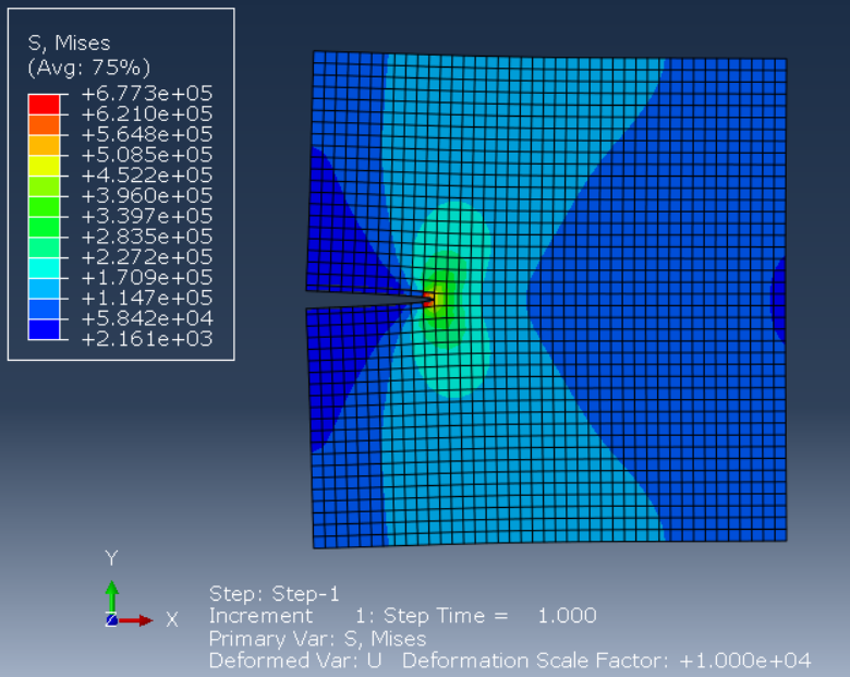
Figure 7: crack propagation in Abaqus

With its ability to handle real-world complexities like multi-physics coupling, dynamic loading, and material nonlinearity, Abaqus remains the preferred choice for engineers seeking accurate and actionable results in failure analysis.

3.2. Initial Steps for Abaqus Crack Analysis

When it comes to fracture mechanics in finite element software, crack propagation, and XFEM are topics you just can’t ignore! While we won’t dive too deep into the details here, we recommend checking out ( Abaqus XFEM Tutorial) for more detailed insights. To model Abaqus crack and perform detailed analyses, you must follow the steps below step by step:

1. Define Material Properties

The first step is to define the material properties. Specify your material’s elastic properties (such as modulus of elasticity and Poisson’s ratio) and plastic properties. For shear materials, defining stress-strain lines is very important.

2. Create Geometry and Meshing

If the crack is in a specific location, design the geometric model and describe its location based on dimensions and constraints. The area near the crack should be meshed more finely and accurately. 

In Abaqus, you can use tools such as XFEM to define the location and shape of the crack. Specify at which surface the crack should exist and under what conditions (such as size and connection to boundaries). An accurate definition of boundary conditions and force laws is of great importance.

3.3. Simulation of Fatigue Crack Growth

Fatigue crack growth is a gradual process where microscopic cracks in a material expand under cyclic loading, potentially leading to catastrophic failure. The simulation of this phenomenon is essential for predicting the lifespan and ensuring the safety of critical structures.

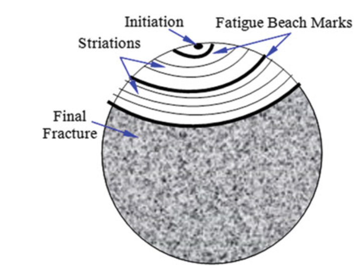
Figure 8: Crack growth zones until final Fracture [Ref]

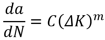
Abaqus, a powerful finite element analysis software, provides advanced tools like the Extended Finite Element Method (XFEM) and cohesive zone models to simulate fatigue crack growth with precision. Central to fatigue analysis is the Paris-Erdogan law, which describes the crack growth rate as a function of the stress intensity factor range :

Here,  represents the crack growth rate, and  are material-specific constants, and  is calculated as . Abaqus uses this relationship to model the propagation of cracks under cyclic loading scenarios, enabling engineers to predict component failure accurately.

The stress intensity factors (SIFs) play a pivotal role in determining crack behavior. For mode I loading, the SIF is calculated as:

Where  is a geometry correction factor,  is the applied stress, and  is the crack length. Abaqus extends this capability to mixed-mode loading, combining mode I and mode II effects. The total energy release rate , which influences crack propagation, is derived as:

Where  is the modulus of elasticity, and  is the mode II stress intensity factor.

Abaqus considers the effect of crack closure, which occurs when the surfaces of a crack come into contact during the unloading phase (when the applied load is reduced). This contact reduces the effective stress intensity range (ΔK), a key factor in predicting crack growth.

The concept of the R-ratio is critical in this context. The R-ratio (R = K_min / K_max) is a measure of the relationship between the minimum stress intensity (K_min) and the maximum stress intensity (K_max) during a loading cycle. For example, in a cycle where the applied load fluctuates between high and low values, K_min represents the lowest stress intensity at the crack tip, and K_max represents the highest. Materials with low R-ratios (where K_min is much smaller than K_max) are more affected by crack closure effects. Abaqus allows users to include experimental data on how sensitive a material is to different R-ratios, enhancing the simulation results’ accuracy and realism.

3.5. Example: Fracture Analysis in Composite Materials Using Abaqus

Composite materials consist of two components: a matrix and a fiber. Combining these two elements can create unique properties for you depending on your intended application. Factors such as the weight percentage of the fibers and the orientation of these fibers play a key role in creating specific mechanical properties. You may need a material in your design that has much higher strength in one direction but not as much in another. Composite materials may be the best answer to these problems. Given the popularity of XFEM in solving fracture problems in Abaqus, let’s utilize this effective method to analyze fracture in composite materials by working through a simple example.

You can learn fracture and crack growth simulation in different types of simulations with different methods in more 7 Examples in our “Abaqus Crack Growth Full Tutorial“.

Consider a composite specimen with the following dimensions. The material of the specimen is carbon/epoxy and the fiber orientation in this material is 0 and 90 degrees. If a crack of a certain length is located in the middle of this specimen, analyze the behavior of the specimen under tensile loading in Abaqus.

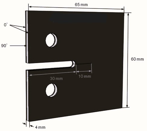
Figure 9: Part dimensions for simulation

Go to the Part module and create a Shell, Extrude (3D) part with a length of 11 and a depth of 6 mm. This part will represent the crack. Then go to the Assembly environment and assemble the created part. Since the depth and length of the crack are greater than the thickness of the sheet, consider a distance of 1 mm in all three dimensions of the part.

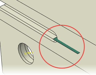
Figure 10: The location of the crack contact with the sample

As stated in the question, the fibers are located in two directions, 0 and 90 degrees. Therefore, it is necessary to define the desired mechanical properties in these two directions. Go to the Property module and define a material named T300/920_90. Follow the path Mechanical → Elasticity in the opened window and select Type: Engineering Constants. Then enter the desired mechanical properties based on the data below.

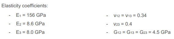
Figure 11: Material properties

Next, to define the failure criterion in the sample, follow the path Mechanical → Damage for Traction Separation Laws → Maxs Damage and complete the desired fields as shown in the image below.

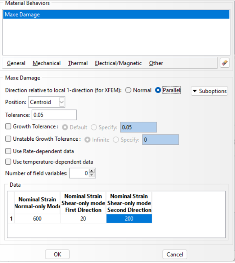
Figure 12: Applying material properties in Abaqus

Then, click on the Suboptions button and select the Damage Evolution option.

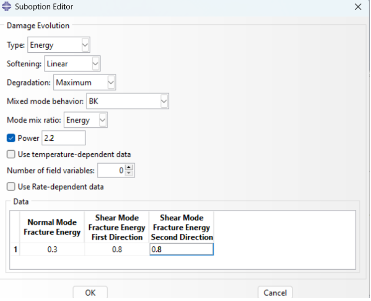
Figure 13: The Damage Evolution option

Again, click on the Suboptions button, select the Damage Stabilization Cohesive option, and enter the value 1e-5 in the window that opens.

Next, create a homogeneous Solid cross-section with the above material and assign it to the sections shown in the figure below.

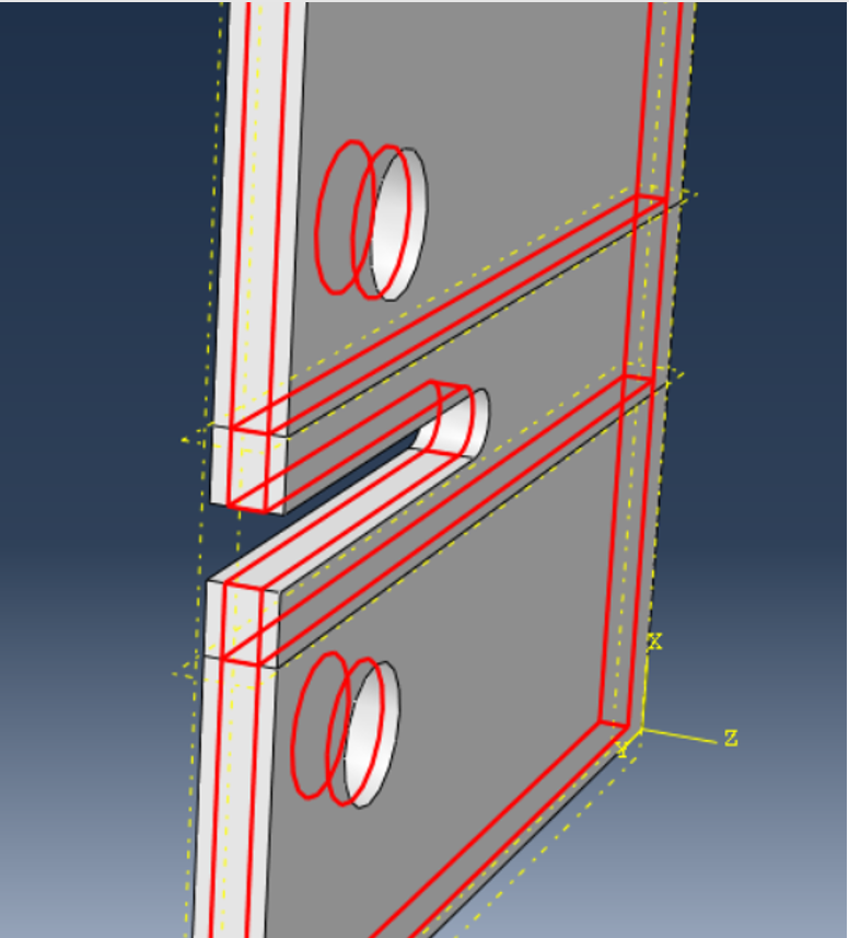
Figure 14: assign the sections

To define the orientation for the material, click on the Assign Material Orientation button and select the area shown in the image above. Then, from the Prompt Area, select “Use Default Orientation or Other Method”.

In the opened window, select Datum csys-1 as the coordinate system and complete the required items as shown in the image below.

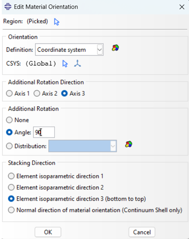
Figure 15: The coordinate system

Now go to the Interaction module and define the crack by going to Special → Crack → Manager in the main menu. To do this, consider the areas indicated in the figure below and select the crack created in the Part module.

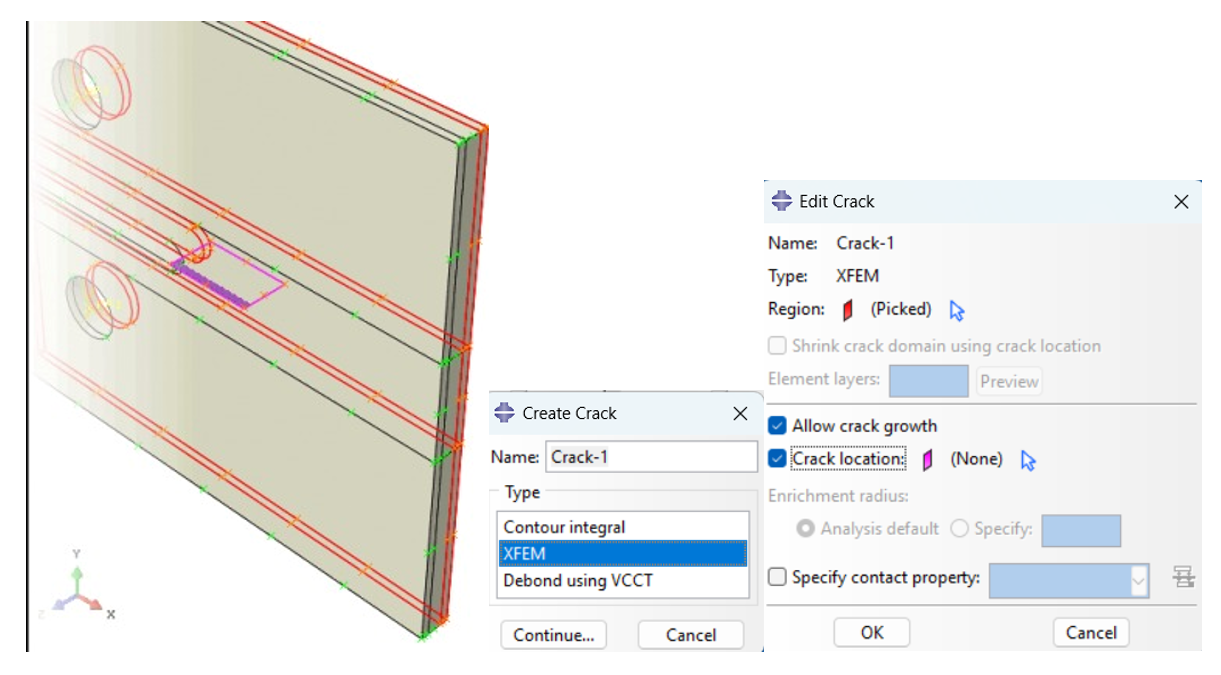
Figure 16: Identifying the crack expansion path

Now you need to repeat the above steps in defining the material for the 0-degree orientation and then define the crack in the remaining areas. After completing the above steps, enter the Step module and define a static, General solver with a time of 1 second, For Convergence Issues, In nonlinear problems (like contact or large deformations), adjusting max increments, step sizes, or tolerances can help Abaqus tackle tricky steps. Optimize speed vs. accuracy by balancing time increments and tweaking mesh settings (adaptive meshing) or stabilization for smoother runs. So then follow the path Other → General Solution Controls → Edit → step-1. Accept the warning that appears and modify the default values ​​using the images below.

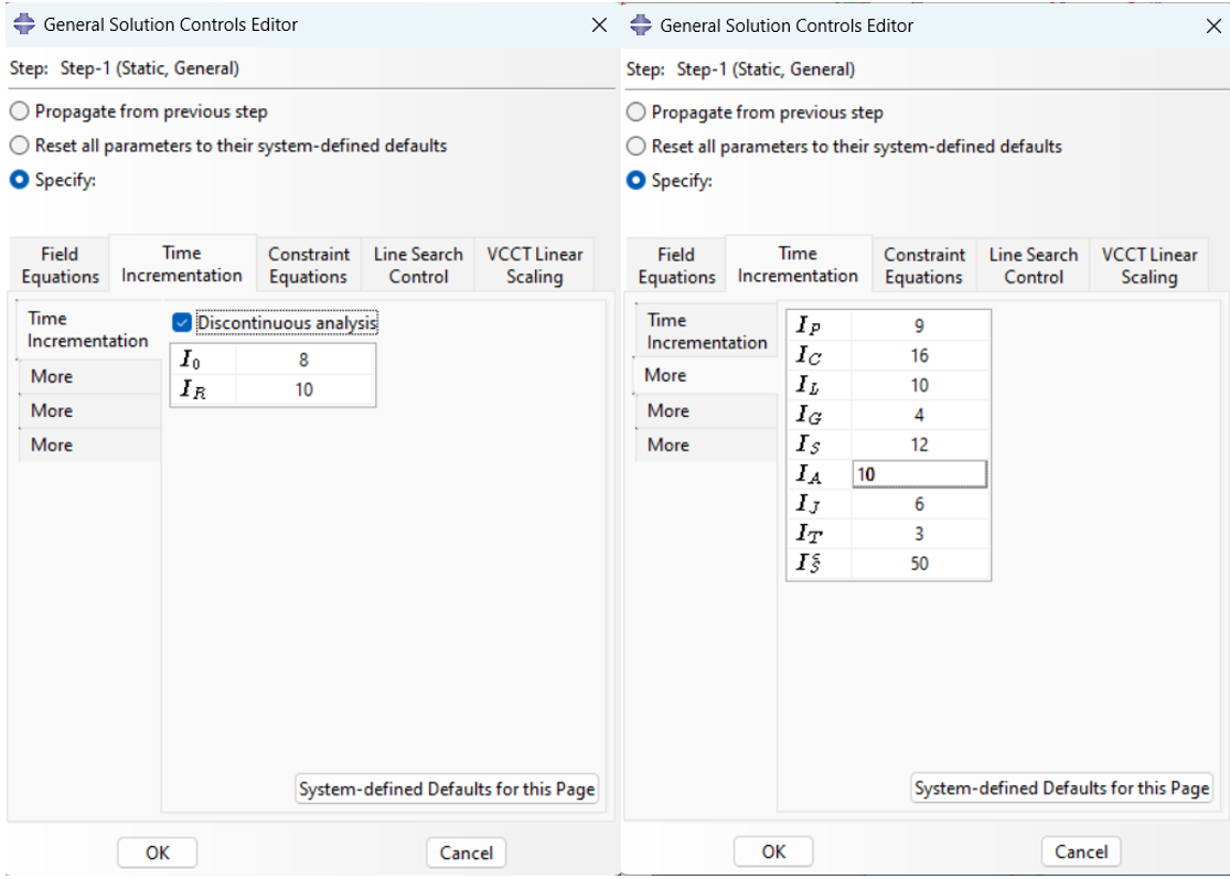
Figure 17: Improving convergence conditions

Then, go to the Load module and apply the movement to the designated points, as shown in the images below.

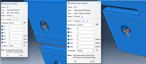
Figure 18: Applying boundary conditions

For meshing, proceed as shown below.

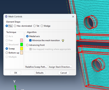
Figure 19: Meshing control

Then send the problem to the Job module for the solution. The image below shows the stress contour in the composite specimen after analysis in Abaqus.

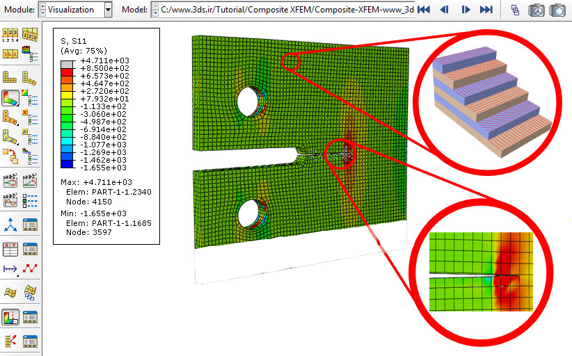
Figure 20: Simulation result

Are you looking to master fracture mechanics and crack modeling in Abaqus? Our comprehensive tutorials offer step-by-step guidance on simulating crack propagation across various materials, including concrete, steel, and bone. With over 300 minutes of detailed video content, these tutorials cover essential methods such as XFEM, J-integral, and H-integral. Also, there are 2D and 3D crack propagation simulation in our tutorial videos.

4. Advanced Applications in Fracture Mechanics

Machine learning is transforming the world of fracture mechanics, bringing new capabilities to simulate and predict crack behavior in materials. By integrating machine learning with fracture simulations, particularly in tools like Abaqus, engineers can now predict crack propagation more accurately, even under complex conditions. This innovative approach allows us to tackle the challenges of anisotropic materials and crack growth, providing new insights into how materials behave under stress. In this section, we’ll explore how machine learning is enhancing fracture mechanics, making predictions more reliable and simulations even more powerful.

 4.1. Integration of Machine Learning with Fracture Simulation

A new aspect of artificial intelligence and machine learning in various industries is the combination of machine learning with fracture mechanics. Let’s step into this new era together and learn about its wonders.

Fracture mechanics, especially in nonlinear cases and complex textures, requires a series of equations and models that can simulate the behavior of cracks in materials with complex geometries and under different loads. In crack modeling, there are always two significant problems:

• Anisotropic behavior of materials: Different materials behave differently under loading, especially at the micro and nanoscale. In this case, the fracture resistance properties change non-uniformly across the material surface.
• Crack propagation: One of the significant challenges in fracture mechanics is the accurate prediction of crack propagation in materials, which requires complex solutions of finite element equations. These equations must include critical stress (K_IC) and plastic parameters near the crack tip.

In this regard, one of the most important aspects is the to predict cracks’ nonlinear and complex behavior and stimulate their development. These predictions can include weak points in the structure, predicting changes in the crack propagation rate, and analyzing the overall strength of structures. Neural networks are one of the most common machine models in this field. These networks can simulate complex relationships between input data and failure. In the field of fracture mechanics, crack characteristics such as loading, geometry, and material properties are fed into the neural network. The neural network can then provide predictions such as crack propagation time, critical locations, and failure probability. For more details and to learn more about neural networks, see our article.

Imagine predicting where a crack will spread in a material before it even forms—or pinpointing the exact stress level that could cause a critical failure. This isn’t science fiction; it’s the cutting-edge synergy of Abaqus simulations and machine learning (ML). Here’s how it works:

Engineers first run fracture mechanics analyses in Abaqus to simulate how materials behave under stress. These simulations generate rich datasets—detailing stresses, strains, displacements, and even the intricate paths of growing cracks. But instead of stopping there, this data becomes the fuel for training ML models. Think of it as teaching an algorithm to recognize patterns: “When stress concentrates here and strain exceeds this threshold, a crack is likely to grow there.” Once trained, these models act like crystal balls for engineers. They can predict crack propagation in new designs, flag risky stress zones in real-time, or even replace time-consuming simulations with lightning-fast ML predictions. For example, an engineer testing a jet engine component could use historical Abaqus data to train a neural network, and then deploy it to assess hundreds of design variations in minutes—not days. The result? Faster innovation, safer products, and a giant leap toward predictive engineering. This fusion of simulation and AI isn’t just smart—it’s the future of how we design resilient materials and structures.

These models can then make more accurate predictions in future simulations, even predicting material performance under unusual conditions that conventional simulations cannot simulate. For example, in an advanced 3D analysis in Abaqus, a machine-learning model can help simulate crack growth in different directions due to geometric changes and loading.

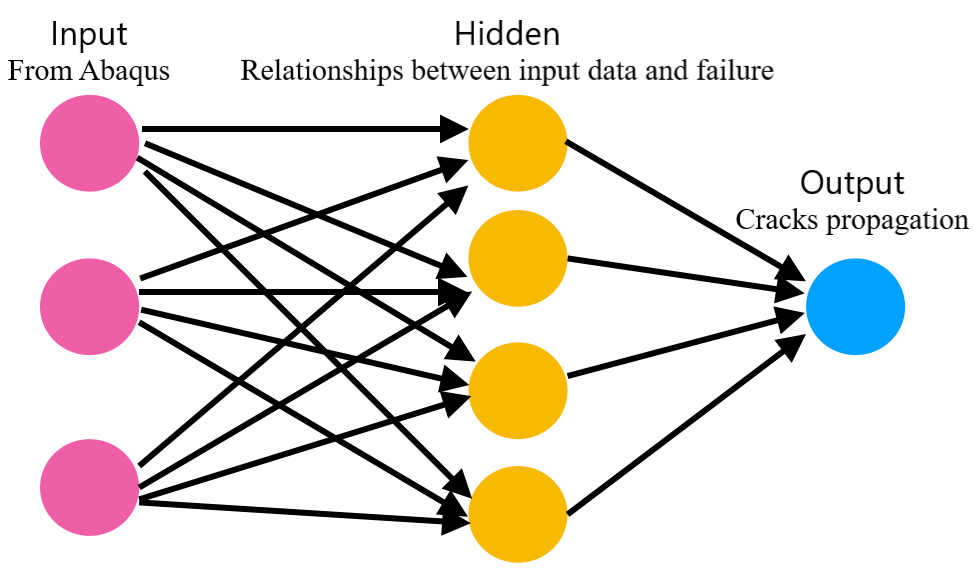
Figure 21: Simple Neural Network

5. Conclusion

This article was written to provide a comprehensive overview of fracture mechanics simulation using Abaqus. It aims to bridge the gap between theoretical principles and practical applications, guiding engineers and researchers in utilizing Abaqus effectively for analyzing crack behavior and preventing structural failures.

The article began by explaining the fundamentals of fracture mechanics, including crack formation and propagation under various conditions. It then explored advanced topics such as Griffith’s theory and fracture modes, emphasizing Abaqus tools like XFEM and cohesive zone modeling. Practical steps for material definition, geometry creation, meshing, and applying boundary conditions in Abaqus were outlined, alongside case studies like fatigue crack growth and composite material analysis. Finally, the integration of machine learning with fracture mechanics was discussed, showcasing the potential for predictive capabilities in complex scenarios.

By combining detailed theoretical insights with practical guidance, this article highlights the power of Abaqus in advancing fracture mechanics studies. It equips readers with the knowledge to perform precise simulations, optimize designs, and address real-world challenges. Returning to the introduction, this article underscores the critical role of fracture mechanics in creating safer, more resilient structures while pointing to the evolving contributions of technologies like machine learning in this vital field.