
Abaqus Topology Optimization 101 | Basics You Must Know

Optimization is a key part of engineering design, helping to improve performance while reducing unnecessary material. In Abaqus, two main types of optimization are available: topology optimization and shape optimization. Topology optimization focuses on finding the best material distribution within a given design space, while shape optimization fine-tunes the structure’s boundaries for better performance.
In this blog, we focus mainly on topology optimization in Abaqus. We explain how it works, how it differs from shape optimization, and walk you through setting up a topology optimization in Abaqus/CAE and through keyword inputs. Whether you are optimizing mechanical components, aerospace structures, or automotive parts, mastering topology optimization in Abaqus can help you create lighter, stronger designs.
Learn structural optimization in Abaqus with our comprehensive tutorials! From foundational concepts to advanced techniques, we cover everything—topology and shape optimization, detailed algorithms, and practical examples with full explanations of settings. Whether you’re starting from scratch or enhancing your skills, these guides have you covered.
|
Full Structural Optimization in Abaqus: Topology + Shape optimization |


1. What is Abaqus Topology Optimization?
An example to illustrate topology optimization is an overweight individual who aims to begin a workout regimen for two primary objectives: to lose weight, or in other terms, to decrease body fat, and to simultaneously build muscle to enhance physical strength, thereby achieving optimal fitness. In this section, we’ll introduce topology optimization concepts in Abaqus briefly and explain their significance in the structural optimization process.
Topology Optimization initiates with a preliminary design, which is regarded as the maximum physical extent of the component. It seeks to establish a new distribution of material by adjusting the density and stiffness of the elements within the initial design while adhering to the optimization constraints. Topology optimization is a mathematical approach that determines the best distribution of material within a given design space. It aims to maximize performance by removing unnecessary material while maintaining structural integrity. The result is often an unconventional, highly efficient design.
To better understand this issue, just take a look at the figure 1. This example of a nonlinear brake pedal illustrates the advancement of a topology optimization process aimed at enhancing stiffness while achieving a 50% reduction in volume.
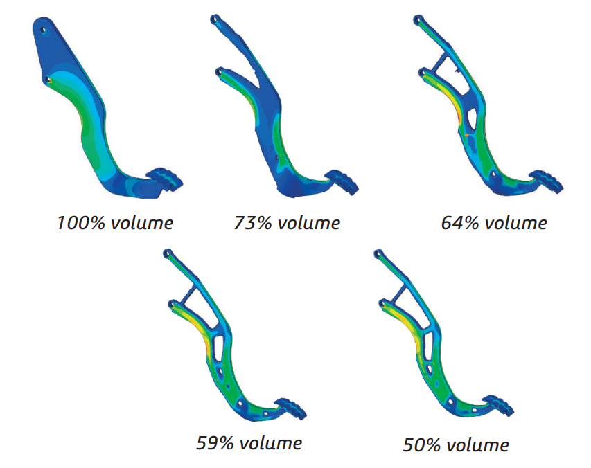
Figure 1: A topology optimization for a brake pedal
Figure 2 depicts the configuration and subsequent processing involved in the topology optimization of a spur gear and shaft assembly utilizing the Abaqus topology optimization module.
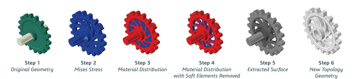
Figure 2: The topology optimization of a spur gear and shaft assembly
1.2. Algorithms of Topology Optimization in Abaqus
Topology optimization encompasses two distinct algorithms:
- The general algorithm: which offers greater flexibility and applicability to a wide range of problems
- The condition-based algorithm: is more efficient but has certain limitations.
By default, the Optimization module employs the general algorithm; however, users have the option to select their preferred algorithm when initiating the optimization task. Each algorithm utilizes a unique methodology for arriving at the optimized solution.
The differences between the topology algorithms are presented in the following table; the table is just an overview! Want to know exactly how these algorithms operates? you can learn that in the Topology Optimization Lesson.
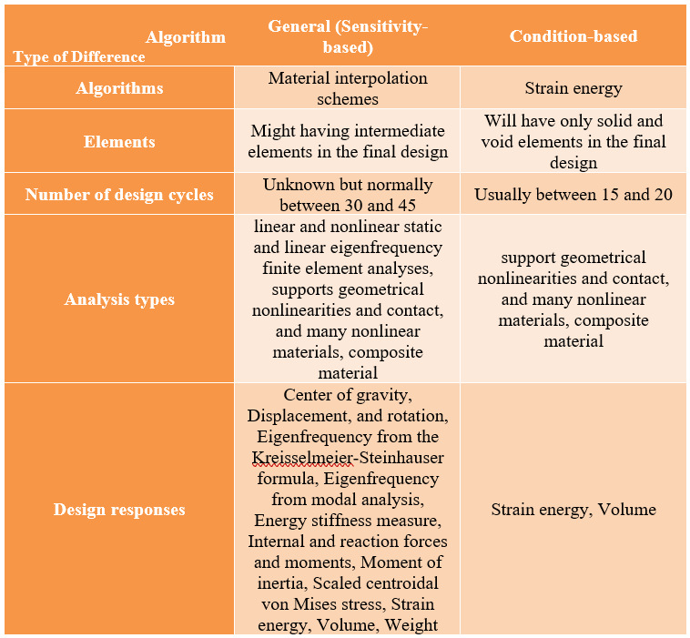
Figure 3: General VS Condition-Based Algorithms
1.3. Topology Optimization Setup in Abaqus
Topology optimization setup in Abaqus includes:
- Defining optimization task: The first step in setting up topology optimization in Abaqus is defining the optimization task, which outlines the overall goal of the optimization process.
- Defining design responses (inputs): Next, you need to define the design responses, which are the inputs. There are the characteristics of the model you want to be changed or better to say to be optimized. The following table shows which design responses can be used as the objective function, constraint, or both.
Did you know that the design responses can be single-term or combined together? Well you can learn all about it in our tutorial.
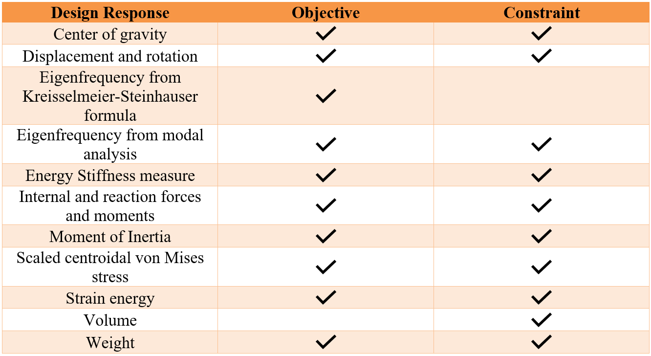
Figure 4: Design Responses of General Algorithm
- Creating objective functions: Afterward, you create objective functions that represent a value that should be either maximized or minimized.
- Creating constraints: Constraints are then created to impose limitations on the design, ensuring the optimized structure meets specific performance or design criteria.
- Creating geometric restrictions: Finally, geometric restrictions are applied to control the shape or size of the design domain, ensuring the solution remains feasible within practical manufacturing limits.
1.4. Applications of Topology Optimization in Engineering Design
Topology optimization in Abaqus is widely used in industries like aerospace, automotive, and civil engineering. It helps create lightweight, strong structures, such as aircraft components, car chassis, and building frameworks, all optimized for performance and material usage.
2. Optimization Process
The optimization process is an iterative procedure that interprets the defined optimization task within the Optimization module of Abaqus. It seeks to identify an optimized solution by evaluating the objective functions and constraints outlined in the optimization task. Figure 5 demonstrates the iterative nature of the optimization process, which involves updating the design variables, adjusting the finite element model, and executing Abaqus analyses in pursuit of an optimized solution.
When you submit an optimization process, this is what happens in every cycle: An Abaqus analysis is performed at first. Next, the optimization module comes in and checks whether the model satisfies the objective functions and constraints; if it doesn’t, then it modifies the model. This is the end of one cycle. The modified model will be analyzed in the next cycle, and then again, the optimization checks it. If the model was not OK, then the optimization module modifies it again and will be analyzed in the next cycle. This routine goes on until the optimization process has converged to an optimal solution or the maximum number of design cycles has been reached.
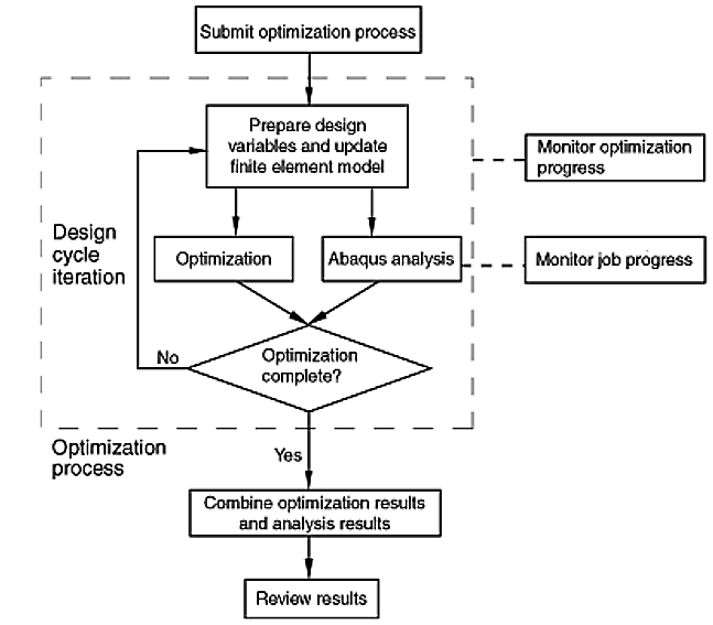
Figure 5: Optimization process
When you want to create an optimization process, when you run it, you must Combine the analysis results and optimization results so you can see the results in the Visualization module of Abaqus!! What? How? Why? Excellent questions. You can find all these answers at the end of the Topology Optimization Lesson.
3. Terminology in Abaqus Optimization
Structural optimization encompasses a unique set of terminology. The subsequent terms are utilized consistently within the Abaqus documentation and the Abaqus/CAE user interface:
- Design Area: The design area refers to the section of your model that is subject to modification through structural optimization.
- Design Response: The inputs to the optimization are called the design responses. In other words, you could say that the design responses are the goals of the optimization; I mean which one of the characteristics of the model you want to be changed or better to say to be optimized.
- Design Variables: In the context of an optimization problem, design variables are the parameters that will be altered during the optimization process.
- Geometric Restrictions: You can also apply geometric and manufacturing constraints that are independent of the optimization; for example, a structure must be able to be cast or stamped or the diameter of a bearing surface cannot be changed.
- Design Cycle: The optimization process is iterative, involving the updating of design variables, conducting an Abaqus analysis on the revised model, and evaluating the results to ascertain whether an optimized solution has been achieved. Each iteration of this optimization is termed a design cycle.
- Optimization Task: An optimization task encompasses the parameters of your optimization, including design responses, objectives, constraints, and geometric limitations.
- Objective Function: It is a quantity that is to be maximized or minimized. These can be single term design responses or combinations of design responses. The objective function is a tool that can maximize or minimize specified design responses.
- Constraints: quantities that will place bounds on the optimization problem (design responses). In other words, Constraints restrict the value of a design response. For example, you want to decrease the mass of the model by 25 percent and the Constraints do this job.
- Stop Conditions: A global stop condition establishes the upper limit on the number of iterations that an optimization process may execute.
The figure below shows the most important concepts of the optimization in Abaqus. You can learn more in detail about other concepts and other settings in the “Introduction optimization” lesson of our tutorial.
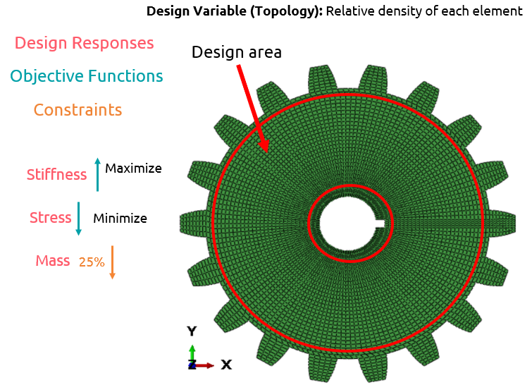
Topology Optimization of a gear in Abaqus. Do you want to learn how to do that? Topology of this gear and more? We have a complete tutorial from the basic and detail settings in our Topology Optimization in Abaqus tutorial.
4. Achieving Precision with Shape Optimization
In this section, we will provide a brief overview of shape optimization concepts and elucidate their importance in the structural optimization process. Shape optimization falls within the domain of optimal control theory. The primary objective is to identify the shape that minimizes a specific cost functional while adhering to established constraints.
4.1. What is Abaqus Shape Optimization?
Abaqus Shape Optimization is employed after the design process, when the overall configuration of a component is established, permitting only slight modifications through the adjustment of surface nodes in designated areas. This process initiates with a finite element model that requires minor enhancements or with a model produced through topology optimization.
The primary aim of shape optimization is to reduce stress concentrations by utilizing the outcomes of stress analysis to alter the surface geometry of a component until the desired stress levels are achieved. An illustration in figure 6 depicts a section at the base of a connecting rod, where surface nodes have been adjusted through shape optimization to mitigate the impact of stress concentration.
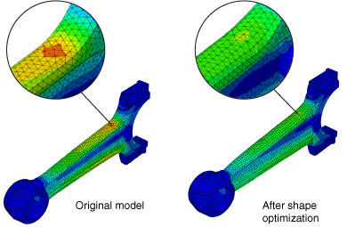
Figure 6: Abaqus Shape Optimization
4.2. Algorithms of Shape Optimization in Abaqus
Shape optimization employs two algorithms:
- The general algorithm
- The condition-based algorithm
The most comment differences between the shape optimization algorithms are in the design responses. More design responses are available in the general than in the condition-based algorithm as shown in figure 7.
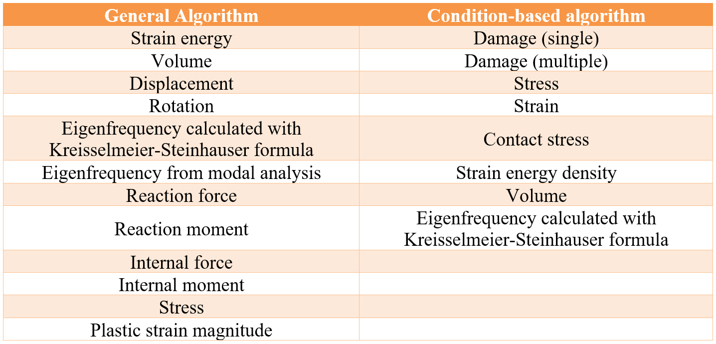
Figure 7: Design responses of shape optimization algorithms
4.3. Shape optimization Setup in Abaqus
Shape optimization setup in Abaqus includes:
- Defining optimization task: The initial step in setting up shape optimization in Abaqus involves defining the optimization task. This task establishes the primary goal of the optimization process.
- Defining design responses (inputs): The next step is to define the design responses, which represent the objectives of the optimization, indicating which specific characteristics of the model you aim to modify or enhance.
- Creating objective functions: At this stage, objective functions refer to a value that is intended to be either maximized or minimized.
- Creating constraints: Constraints are then introduced to define the permissible range of a design response.
- Creating geometric restrictions: Finally, geometric restrictions are imposed to regulate the shape or size of the design domain, ensuring that the final solution remains feasible for practical manufacturing. More you can understand of geometric restrictions in Shape Optimization Lesson of our tutorial.
- Creating stop conditions: Stop conditions are defined to determine when the optimization process should be halted, typically based on criteria such as reaching a maximum number of iterations, achieving a desired level of convergence, or meeting specific performance targets.
4.4. Advantages of Shape Optimization in Abaqus
Abaqus offers powerful shape optimization tools that allow for precise control over the design geometry. Engineers can fine-tune the shape to ensure it performs optimally under various conditions, making Abaqus an invaluable tool for enhancing structural performance. Shape optimization can be used to fine-tune a design, allowing engineers to refine their designs for maximum performance and efficiency.
5. How Topology and Shape Optimization Work Together
While both topology and shape optimization can be performed separately, they often work best when combined. Topology optimization is used to create a lightweight structure by finding the optimal material distribution, while shape optimization is used to fine-tune the outer geometry for better performance. The synergy between topology and shape optimization allows engineers to create structures that are both lightweight and strong, with optimized material distribution and geometry. This combined approach is particularly useful in industries like aerospace and automotive engineering.
5.1. Practical Examples of Combined Optimization Techniques
For example, in aerospace, a wing component may first undergo topology optimization to reduce weight and material usage. The resulting design can then be refined using shape optimization to ensure it is aerodynamically efficient, robust, and manufacturable. In Abaqus, this combination results in a design that performs at peak efficiency, with optimized material usage and an aerodynamic shape.
6. Step-by-Step Guide to Running Optimization Simulations in Abaqus
It should be noted that install TOSCA structure software before starting the optimization process in Abaqus. There are various steps to running optimization simulations in Abaqus. Figure 8 shows the user actions and Abaqus actions in the optimization process.
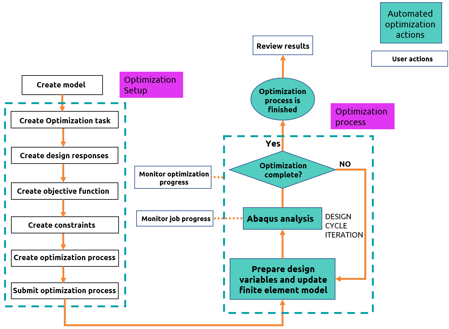
Figure 8: User actions and automated Abaqus actions in the optimization process
Here’s a detailed guide to running optimization simulations in Abaqus:
6.1. Preparing Your Model for Optimization
Before running an optimization simulation in Abaqus, ensure that your model is properly set up. This includes defining material properties, boundary conditions, and loading conditions. Additionally, identify the optimization objectives and constraints that will guide the design process. It is worth mentioning that you should run a complete analysis of your model and make sure that it runs to completion before you attempt to run an optimization process.
6.2. Setting Up and Defining Optimization Parameters
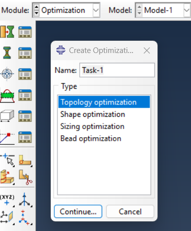
Once the model is ready, define the optimization parameters in Abaqus. As shown in figure 9 (from left to right, respectively), this includes selecting:
(a) Type of optimization task,
(b) Design Response,
(c) Objective functions,
(d) Constraint,
(e) Create optimization process,
(f) Submit the optimization process.
(a)
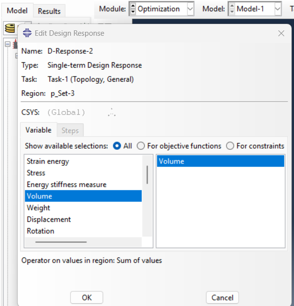
(b)
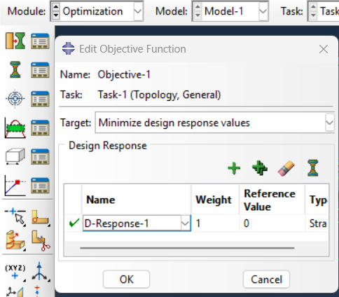
(c)
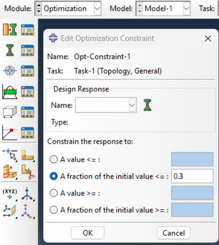
(d)
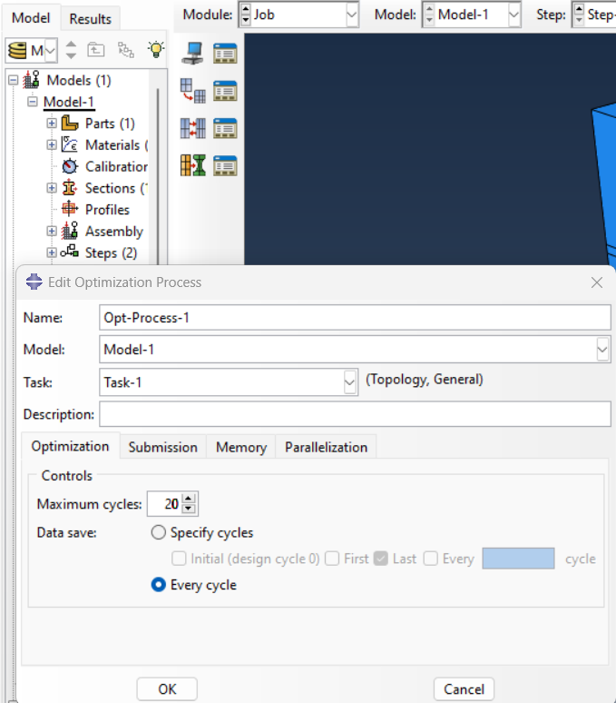
(e)
Figure 9: Defining optimization parameters in Abaqus
If you look at the figure above, you can see that there are a lot of settings for each window and each step; seems overwhelming, right? well we have explained them all in detail and how they operates in our tutorial.
6.3. Interpreting Results from Optimization Simulations
After running the optimization simulation, Abaqus provides results that show the optimized design (See figure 10). It’s essential to carefully interpret these results to assess whether the design meets all performance, safety, and material-use goals. Adjustments can be made based on these results to fine-tune the design.
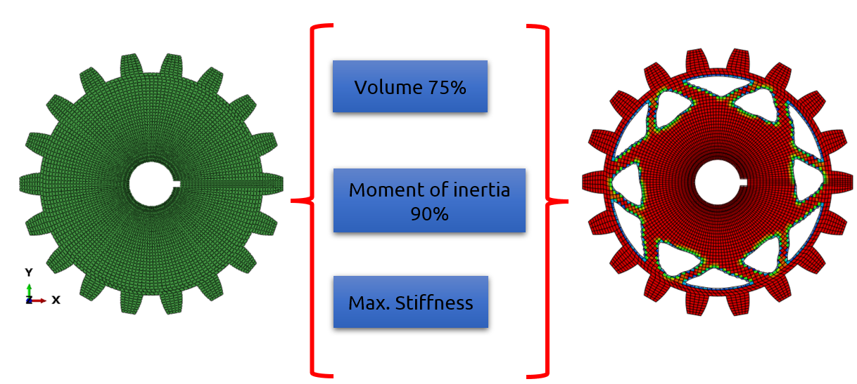
Figure 10: Schematics of results from optimization simulations
7. A Practical Example: Bridge Optimization in Abaqus
In this section, a practical example will be explained to learn how to use the topology optimization module in Abaqus. Let’s consider a steel bridge structure that needs to be optimized for material efficiency and strength (Left side of figure 11). The goal is to create a lightweight, cost-effective bridge design that can handle the expected loads without compromising safety (Figures 11 and 12).
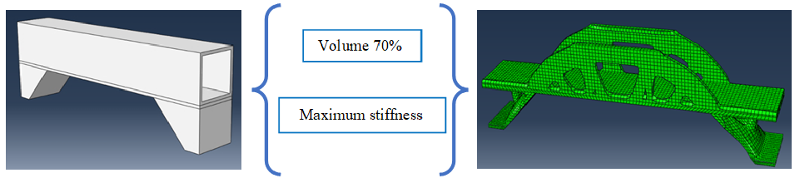
Figure 11: Problem objectives
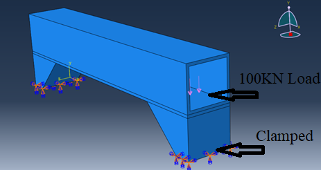
Figure 12: Problem boundary conditions
7.1. How to Model the Bridge
Model the bridge in Abaqus by defining its geometry. Assign properties such as steel’s density (7850 kg/m³) and Young’s modulus (210 GPa). Define loading conditions as clamped supported (Figure 12). Ensure that the model represents the key aspects of the bridge’s design, such as supports, spans, and load-bearing components. Then use the appropriate mesh (Figure 13).
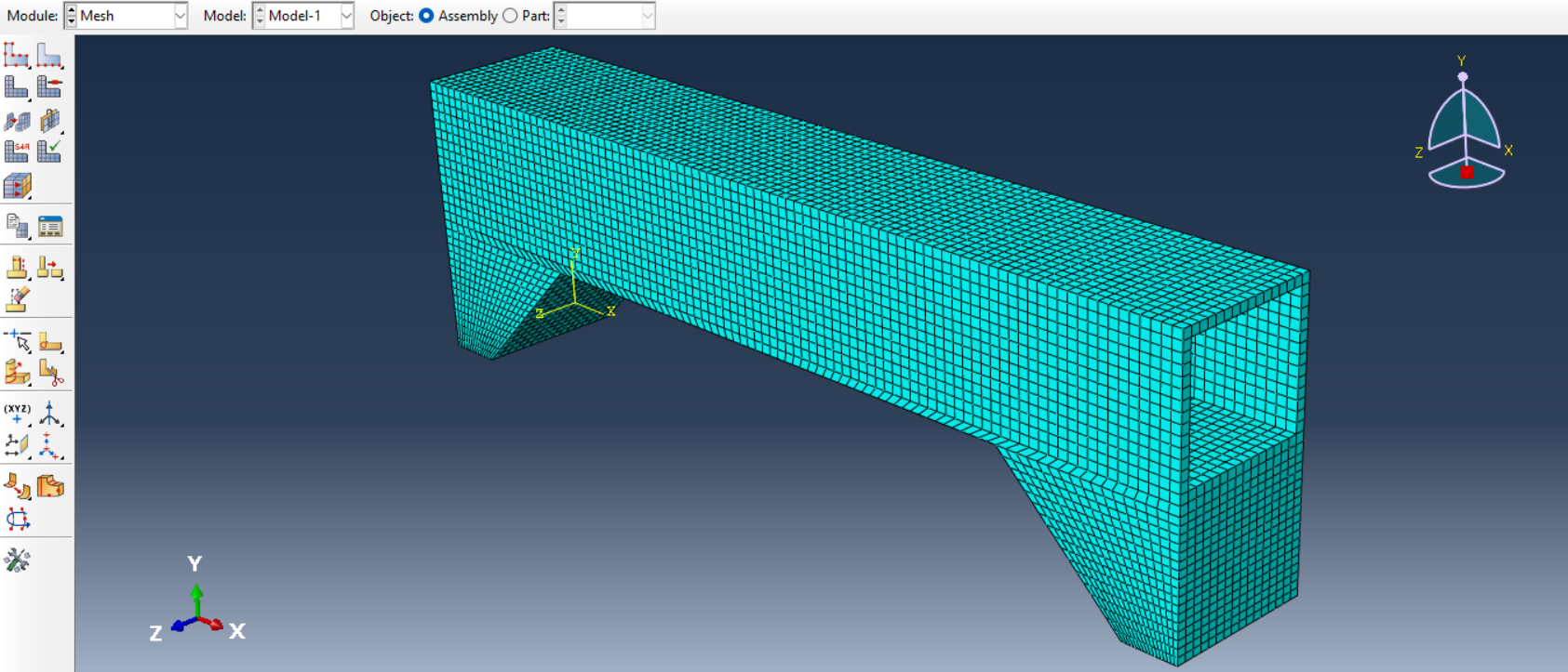
Figure 13: Meshing the bridge
7.2. Run without optimization
First, you should run the static problem and check the results as shown in figure 14. As you see, maximum torsion is equal to 2 Mpa in some regions. Now we want to reduce the weight of the bridge and maximize the stiffness.
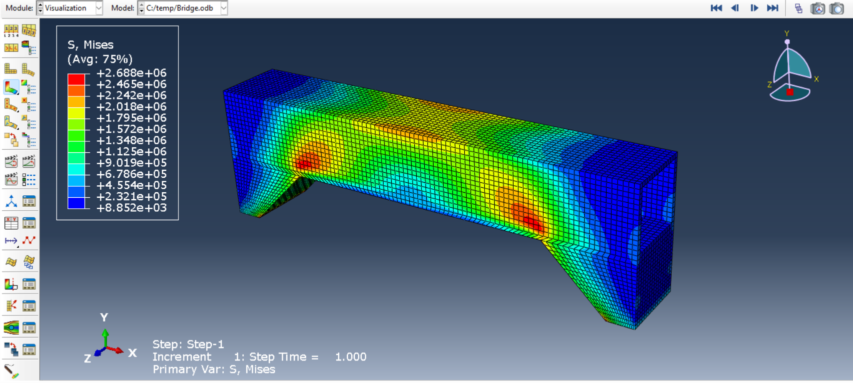
Figure 14: Stress results from the static analysis
7.3. How to Run an Optimization Task in Abaqus
Set up an optimization task in Abaqus by choosing topology optimization and defining the appropriate constraints and objectives (See figure 15).
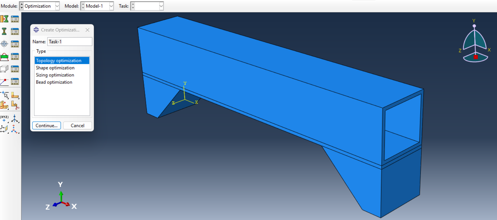
Figure 15: Choosing topology optimization task
To not have any changes in load and boundary conditions, you can select the two options shown in Figure 16. By selecting these options, you can freeze load and boundary conditions regions.
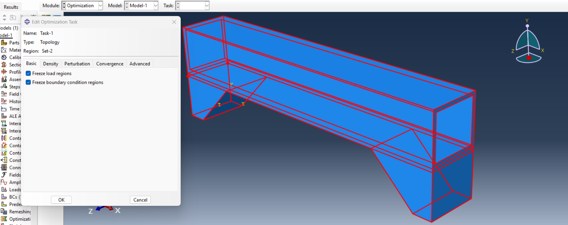
Figure 16: Freezing loading and boundary conditions
Create a constraint for the volume. Enter 0.3 for the fractional of the initial value to decrease volume to 30 percent (See figure 17). It should be noted that the geometry restrictions must be applied so that there is no problem during manufacturing. But in this example, geometry restriction is not considered.
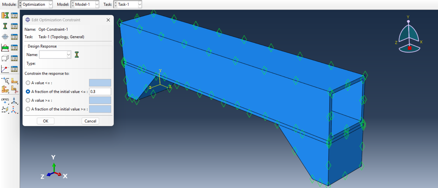
Figure 17: Define the volume reduction percentage
Create an optimization process with a maximum cycle of 20 and save it for every cycle (See figure 18).
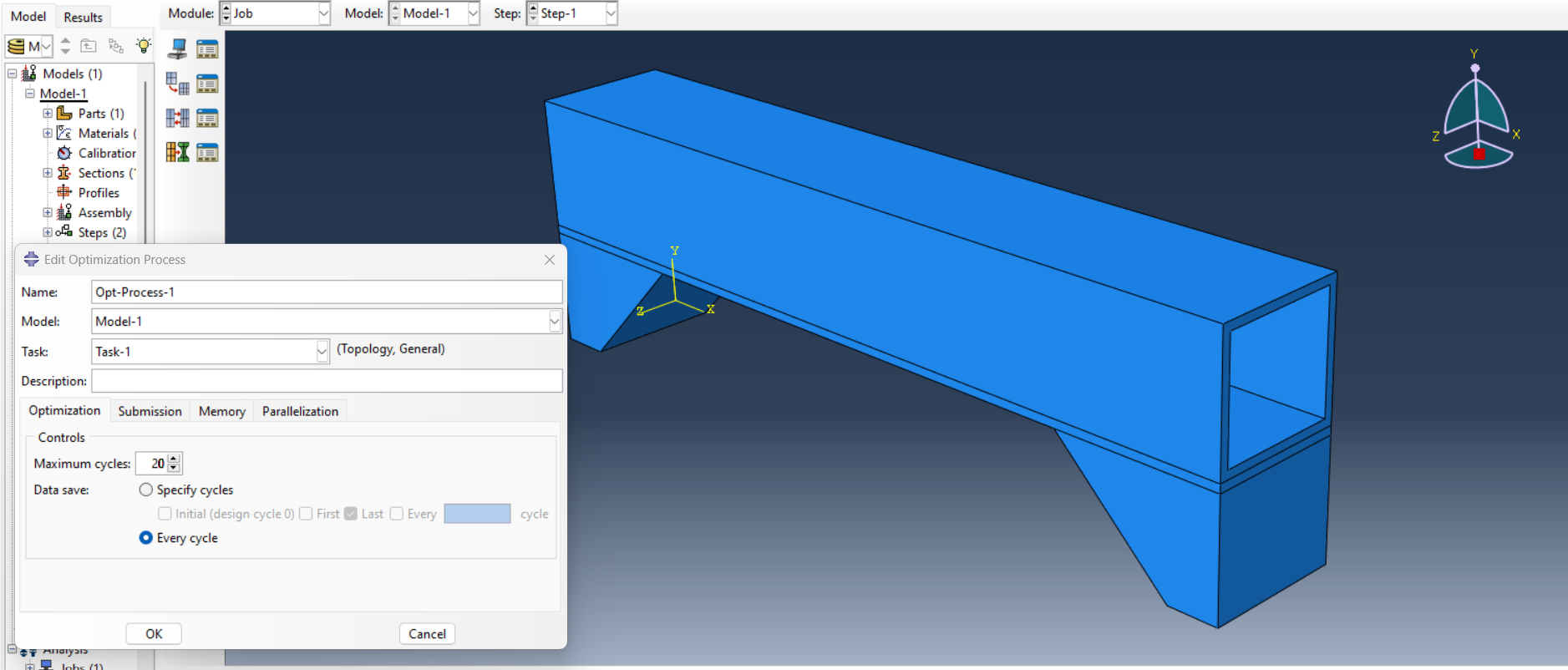
Figure 18: Creating optimization process and defining the maximum design cycle
Run the simulation and evaluate the results, making adjustments as needed to meet the design goals (See figures 19 and 20).
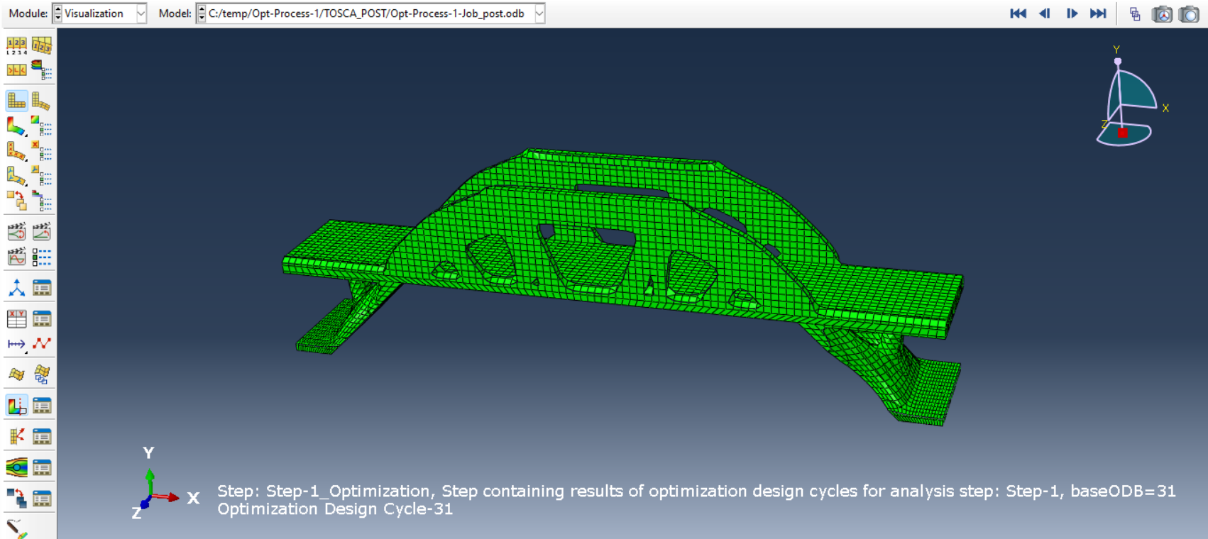
Figure 19: The optimized bridge
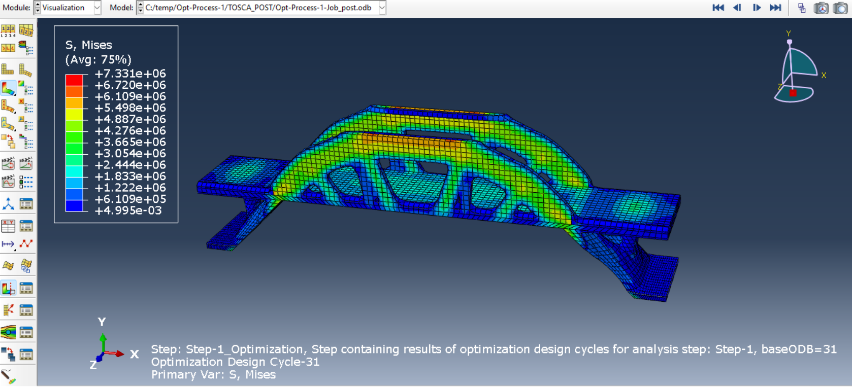
Figure 20: Stress contour of the optimized bridge
8. Common Challenges in Topology and Shape Optimization (And How to Overcome Them)
While optimization in Abaqus offers incredible benefits, it’s not without its challenges. Some common issues include:
- Convergence Issues and Solution Strategies
One of the challenges in optimization is ensuring that the solution converges to a feasible and optimal design. Adjusting parameters such as mesh density, solver settings, and boundary conditions can help address convergence issues.
- Handling Complex Geometries and Constraints
Complex geometries and constraints can complicate the optimization process. Simplifying the design or applying advanced meshing techniques in Abaqus can help overcome these challenges.
- Managing Computational Resources Effectively
Optimization simulations can be computationally intensive. By using high-performance computing resources and optimizing the simulation setup in Abaqus, engineers can manage computational resources effectively and reduce processing times.
By understanding these challenges and applying best practices, such as carefully selecting constraints and verifying results with physical tests, engineers can overcome these hurdles and achieve optimized designs.
9. Case Studies: Real-World Applications of Optimization in Abaqus
Optimization in Abaqus finds application in various domains, including the automotive industry, aerospace industry, and civil engineering.
- Automotive Industry: Lightweight Component Design
Abaqus is widely used in the automotive industry to design lightweight components, such as chassis and suspension parts (See figure 26). Topology optimization helps create stronger, lighter components that improve fuel efficiency and safety.
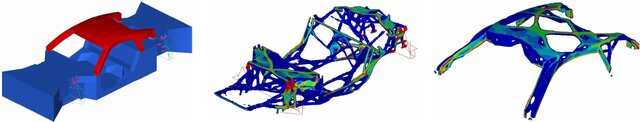
Figure 21: Automotive chassis topology optimization
- Aerospace Industry: Structural Integrity and Weight Reduction
In the aerospace industry, optimization techniques in Abaqus are used to design lightweight yet strong aircraft structures, reducing fuel consumption and improving performance (See figure 22).
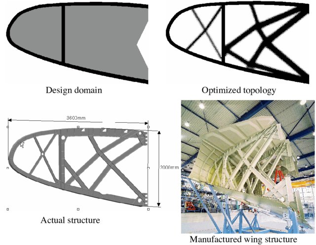
Figure 22: The resulting topology, actual design, and manufactured the front part of an airplane wing
- Civil Engineering: Optimizing Building and Bridge Structures
In civil engineering, Abaqus enables the optimization of large-scale structures, such as bridges and buildings, ensuring they are both efficient and durable.
5. Conclusion
In this blog post, we discussed optimization techniques available in Abaqus, with a focus on topology optimization. We reviewed the basic difference between topology and shape optimization: topology optimization adjusts the material layout, while shape optimization refines the structure’s boundaries. Understanding these differences is important when choosing the right method for your project.
We then showed how to perform a topology optimization in Abaqus, both through the CAE interface and using keywords. With topology optimization, engineers can achieve lighter, more efficient designs while maintaining strength and performance. By learning how to set up and control the optimization process in Abaqus, you can improve your simulations and reach better design outcomes.