
Concrete Simulation in Abaqus | Reinforced Concrete Models
Most modern buildings, bridges, and tunnels are built with reinforced concrete. It’s a key material in structural engineering because it combines the compressive strength of concrete with the tensile strength of steel. This combination makes reinforced concrete ideal for handling different types of loads.
To design safe and reliable structures, engineers use concrete simulation tools. One of the most powerful tools for this is Abaqus. With it, you can run detailed finite element analysis of reinforced concrete structures. This helps predict how the structure will perform under real-world conditions.
In this blog, you’ll learn how to use Abaqus concrete tools to model reinforcement. We’ll explain key methods like rebar layers and the embedded region technique. You’ll also see how to simulate failure using models like CDP and traction-separation laws. Whether you’re doing concrete structural analysis or designing a new beam or slab, this guide will help you do it right.
What is included in this package?
Workshops
Files
The topics in this package include, but are not limited to: concrete, beam-column structures, composites, steel rebars, Ultra-High-Performance-Fiber-Reinforcement Concrete columns, CFRP bars, etc.
1. What is Reinforced Concrete?
Reinforced concrete is a composite material. It combines concrete’s ability to resist compression with the tensile strength of steel bars or meshes. These two materials work together to handle different forces in a structure.
The reinforcement is placed inside the concrete before it sets. This bond allows them to act as a single unit when loads are applied. As a result, the structure becomes stronger and more flexible. It can now resist tensile and shear forces that plain concrete cannot handle on its own.
Reinforced concrete is utilized in many structures due to its versatility and strength. Some examples include buildings, and bridges as beams, columns, and foundations.
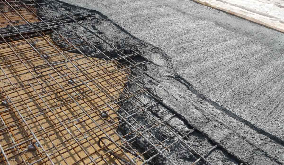
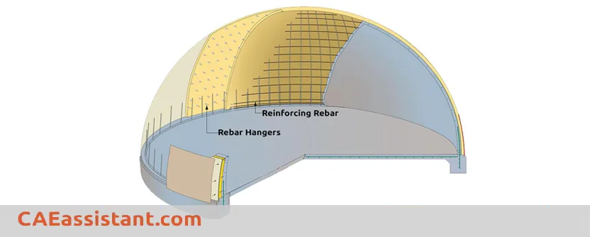
Figure 1: Reinforced Concrete Foundation [Ref]
2. Finite Element Analysis of Reinforced Concrete Structures
Finite element analysis of reinforced concrete structures is a powerful way to understand how buildings and infrastructure respond to loads. This method breaks down complex geometry into smaller parts (finite elements) to simulate stress, strain, and deformation.
Reinforced concrete shows nonlinear behavior due to cracking, crushing, and yielding. These factors make accurate modeling essential. With tools like Abaqus concrete, engineers can simulate these effects using detailed material models.
One key model in concrete structural analysis is the Concrete Damaged Plasticity (CDP) model. It captures both the damage and plastic behavior of concrete. Abaqus also supports features like tension stiffening, bond-slip, and cyclic loading—critical in seismic design. This makes finite element analysis of reinforced concrete structures an essential tool for safe and efficient design.
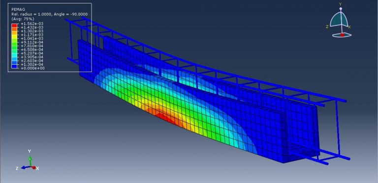
Figure 2: A reinforced concrete beam under a three-point bending test
In the following sections, we will delve deeper into the methodologies and considerations involved in the finite element modeling of reinforced concrete structures, providing insights into best practices and common challenges.
3. How to Reinforce the Concrete in Abaqus? | Abaqus Concrete Simulation
When doing concrete simulation in Abaqus, it’s important to model both concrete and steel reinforcement accurately. Depending on the structure and the level of detail needed, Abaqus offers several methods to simulate this interaction.
Two Common Techniques for Reinforced Concrete Modeling:
3.1. Rebar Layers in Shell or Membrane Elements
This method works well for thin elements like slabs, walls, and panels. Instead of modeling steel bars as separate parts, they are added as layers within shell or membrane elements. You define material properties, orientation, and spacing. This makes the model simpler and reduces simulation time.
3.2. Embedded Region Method in Solid Elements
For more detailed concrete structure analysis, the embedded region method is often used. Here, steel bars are created as wire or truss elements and embedded into solid concrete elements. Abaqus uses constraints to link them. This gives a more realistic simulation, especially when analyzing local stress or failure.
Each approach has its pros and cons. For example, research indicates that accurately modeling the bond-slip effect between reinforcement and concrete is essential for realistic simulations—an important factor in finite element analysis of reinforced concrete structures. The embedded region method can capture this behavior more effectively than rebar layers. These methods are fully explained in the next parts.
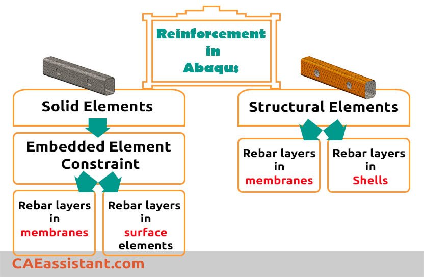
Figure 3: Reinforced concrete simulation methods in Abaqus
Note: there are seven practical examples about modeling reinforced concrete in Abaqus in our full tutorial concrete package; three of them are:
- Dynamic compression test of in concrete column reinforced with CFRP bars
- Finite element Analysis of hollow-core square reinforced concrete columns wrapped with CFRP under compression
- Axial compression in the damaged CFRP reinforced concrete column with initial residual stress
You can learn more about columns and beams and the difference between them in this blog: “Concrete Column Analysis + Beams Explained: Design, FEA“
4. Using Structural Elements to specify Rebar Layers | Abaqus Rebar
In Abaqus concrete modeling, rebar layers can be added to structural elements like shells, membranes, or surfaces. This method is especially useful for thin-walled components such as slabs and walls, where reinforcement is mostly in one direction.
Advantages of Using Rebar Layers
-
Efficient for Thin Structures
Rebar layers simplify modeling for elements like slabs, reducing complexity and saving time. -
Separate Material Behavior
The reinforcement has its own material properties, separate from the host element. This helps simulate composite behavior more accurately. -
Lower Computational Cost
Since rebars aren’t modeled as full 3D parts, analysis runs faster and uses fewer resources. -
Detailed Control in Shell Elements
You can define bar size, spacing, orientation, and even vary these within a single element. This allows for advanced concrete simulation with non-uniform reinforcement. -
Clear Stress Visualization
Abaqus shows results for each rebar layer, helping engineers understand stress distribution in reinforced areas.
Limitations of Rebar Layers
-
Limited to Shell-Type Elements
Rebar layers only work in shell, membrane, or surface elements. They’re not suitable for full 3D models. -
Low Volume Fraction Only
Best used when reinforcement volume is low—typically between 1% and 4%. -
Simplified Bond Behavior
The method doesn’t fully capture bond-slip effects between steel and concrete. -
Assumes Uniform Layout
Rebar layers assume a regular bar distribution, which might not reflect complex reinforcement designs. -
Challenging for Shear Reinforcement
Modeling stirrups or other shear reinforcements can be more difficult with this approach.
This method offers a balanced trade-off between modeling speed and structural accuracy—especially useful in early stages of concrete structural analysis.
If you do not know the difference between shell and membrane elements, look at this blog:
What is the difference between membrane and shell elements?
Surface elements do not have any element properties other than the rebar layer. In other words, they are used primarily just as placeholders for rebar layers.
4.1. Defining rebar layers in Abaqus/CAE | rebar modeling
In Abaqus concrete modeling, rebar layers are used to simulate uniaxial reinforcement in shell, membrane, or surface elements. These layers behave independently from the host element, making them ideal for accurate concrete simulation in thin structures.
Use rebar layers when the reinforcement volume is small (typically under 4%). Since the volume of the rebar is not subtracted from the host element, this approach works best for lightweight reinforcement.
Now let’s see how to define rebar layers:
1. From the Options field of the shell, membrane, or surface section editor, click the Rebar Layers… icon. The Abaqus Rebar Layers dialog box appears.
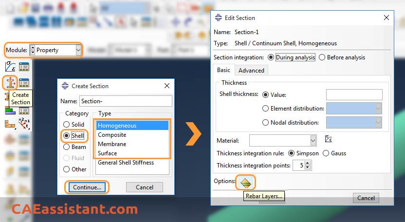
Figure 4: Selecting the Rebar Layers option in Abaqus
2. Set Geometry Type
-
Constant: Use this for evenly spaced bars.
-
Angular: Use this if the rebar spacing varies as a function of radial position in a cylindrical coordinate system.
3. Fill in the Layer Details
In the dialog box, enter data for each layer:
- Name: the name of the rebar layer (to identify the layer in the list of section points when post-processing in the Visualization module).
- Material: the name of the material forming the rebar layer. Click the arrow that appears to display the list of available materials, and select the material you created before forming the rebar layer.
- Area: the cross-sectional area per bar.
- Spacing: the rebar spacing in the plane of the section. For angular rebar spacing, specify the spacing angle in degrees.
- Orientation: the angular orientation of the rebar (in degrees) relative to the 1-direction of the rebar reference orientation.
- Position (not applicable for membrane/surface): the position in the shell thickness direction measured from the middle surface of the shell.
This setup allows for flexible and detailed modeling during finite element analysis of reinforced concrete structures.
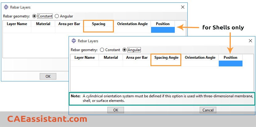
Figure 5: Rebar Layers dialog in Abaqus
Specifying rebar geometry
When setting up rebar layers in Abaqus concrete models, it’s important to define their geometry correctly. Rebar geometry is always defined relative to a local coordinate system.
Two Geometry Options
-
Constant Geometry
Rebars are spaced evenly. This is the most common option and works well for flat or regular structures. -
Angular Geometry
Use this when the bar layout changes with radial position—ideal for cylindrical or circular elements.
Key Parameters to Specify
-
Spacing (s): Distance between the bars, either linear or angular depending on the geometry type.
-
Angular Orientation (α): Direction of the rebar relative to the local coordinate system. This helps control how the bars resist loads within the element.
Correctly defining rebar geometry improves the accuracy of concrete structural analysis and helps represent real-world behavior more closely.
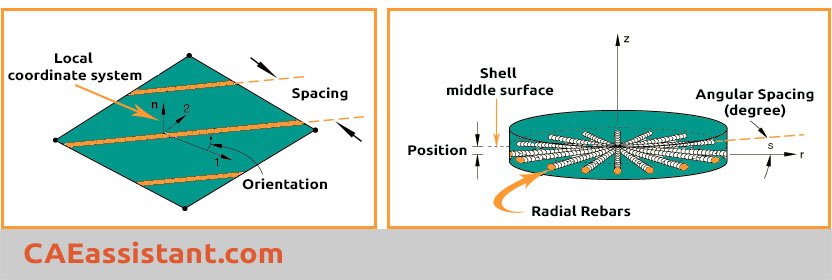
Figure 6: Specifying rebar spacing and angular orientation
Output for rebar elements
Abaqus/CAE supports visualization of rebar layer orientations and results in rebar layers. The output of variables such as stresses and strains at the rebar integration points is available on a layer-by-layer basis. Remember to request outputs for rebars when defining a step:
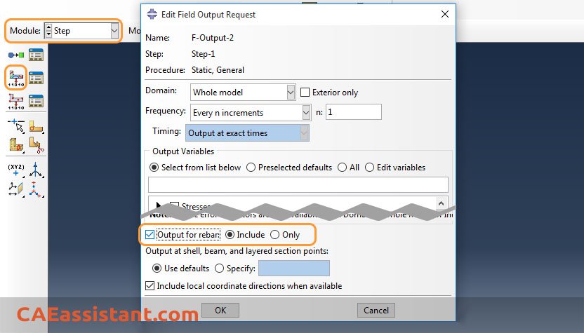
Figure 7: Defining output for rebar element
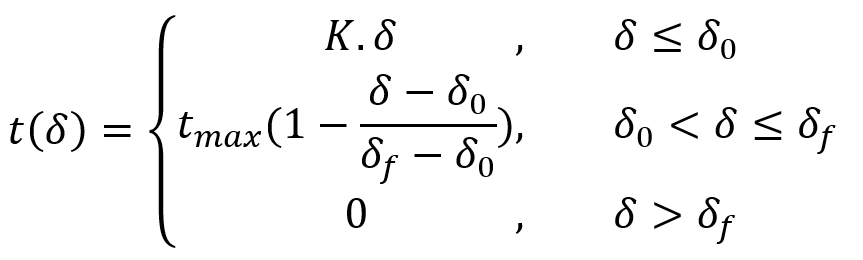
5. What is Abaqus Embedded Region?
The embedded region technique in Abaqus is a modeling strategy used to simulate composite materials or structures where one region (the embedded region) is entirely enclosed within another (the host region). In the context of reinforced concrete, this method allows for the integration of reinforcement elements (such as rebar layers defined in shell or membrane elements) within a solid concrete matrix.
By using this technique, the degrees of freedom of the embedded nodes are constrained to follow the deformation of the host elements. This approach facilitates the independent meshing of reinforcement and concrete elements, simplifying the modeling process and ensuring an accurate representation of the composite behavior.
- Embedded region components:
- Embedded region:This is the inner region, often representing reinforcement or inclusions in a material. For instance, fibers in a composite or rebar in concrete.
- Host region:This is the outer region that surrounds the embedded region. It typically represents the matrix material in a composite or concrete.
- Benefits:
- Simpler mesh generation compared to directly creating a combined geometry.
- Preserves material properties assigned to each region.
- Well-suited for applying periodic boundary conditions elements.
What is included in this package?
Workshops
Files
The topics in this package include, but are not limited to: concrete, beam-column structures, composites, steel rebars, Ultra-High-Performance-Fiber-Reinforcement Concrete columns, CFRP bars, etc.
6. Using Rebar layers in Solid elements
To model reinforcement within solid concrete elements using rebar layers, follow these steps:
- Define Rebar Layers on Structural Elements: Begin by creating shell, membrane, or surface elements and assign rebar layers to them. These structural elements represent the reinforcement within the model.
- Embed Structural Elements into Solid Elements: Use the embedded region constraint to embed the rebar-defined structural elements into the solid concrete elements. This method allows the reinforcement to interact appropriately with the concrete matrix without the need for matching meshes.
This approach is particularly advantageous when dealing with complex reinforcement layouts or when a detailed representation of the reinforcement is required within a solid concrete structure.
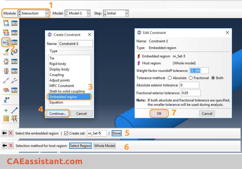
Figure 8: Embedded region constraint in Abaqus
When selecting the Whole Model, Abaqus searches the elements in the vicinity of the embedded elements for elements that contain embedded nodes. After that, the embedded nodes are constrained by the response of these host elements. To preclude certain elements from constraining the embedded nodes, you can define a host element set (Select Region).
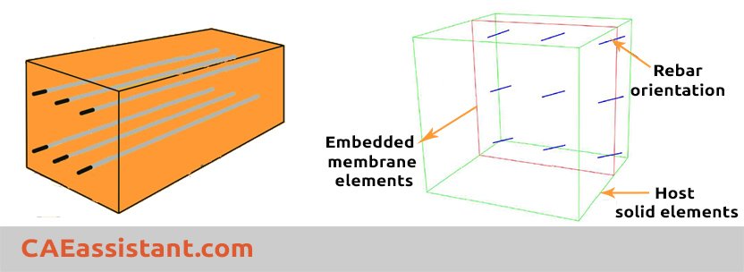
Figure 9: Embedded region components
7. Concrete Structural Analysis: Reinforced Concrete Failure Models
In concrete structural analysis, it’s crucial to understand how reinforced concrete fails. The interaction between concrete and steel reinforcement makes the behavior complex—especially under varying loads. To simulate this accurately, Abaqus offers several failure models.
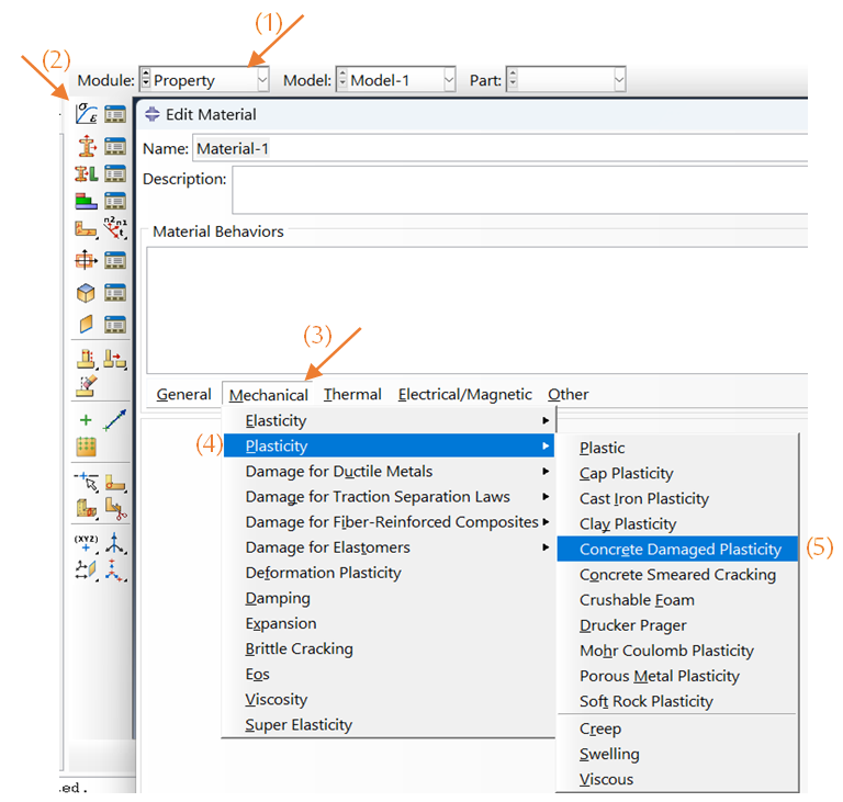
1. Concrete Damaged Plasticity (CDP) Model
The Concrete Damaged Plasticity (CDP) model is widely used in Abaqus concrete simulations. It captures both tensile cracking and compressive crushing by combining damage mechanics with plasticity.
Key Features:
-
Simulates tension and compression failure mechanisms separately
-
Works for static, cyclic, and dynamic loading
-
Includes stiffness degradation and irreversible strain
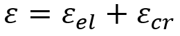
The model uses a stress-strain relationship that accounts for elastic, plastic, and damaged behavior. You can find the CDP option in the Property module of Abaqus.
Figure 10: defining CDP model in Abaqus Property module
For a deeper dive into CDP, see our full guide: “Concrete Damage Plasticity (CDP) in Abaqus.”
2. Smeared Crack Model
The smeared crack approach treats cracks as a spread-out strain across elements, not as sharp breaks. This makes it suitable for general concrete simulation, especially when crack paths aren’t the main focus.
Key Features:
-
Reduces stiffness in cracked directions
-
Good for distributed cracking behavior
-
Avoids tracking individual crack surfaces
The strain is split into elastic and cracking parts, allowing a smooth simulation of crack effects.
Formulation:
The total strain is decomposed into elastic and cracking components:
Where:
 is the total strain
 is elastic strain
 is cracking strain
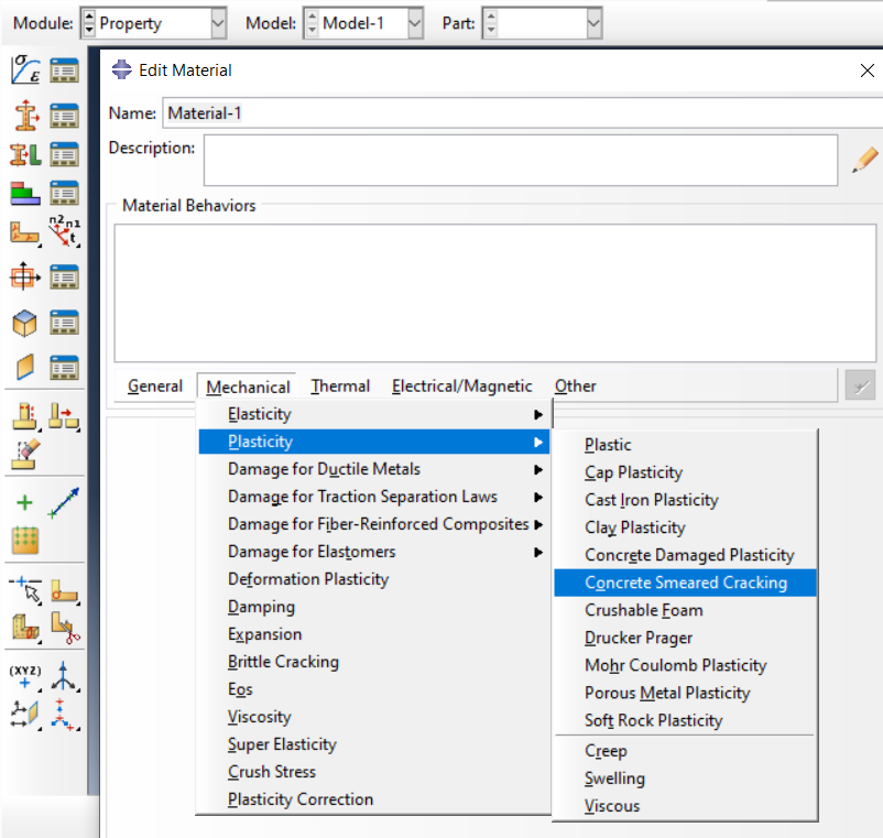
Figure 11: Defining Smeared crack model in Abaqus
3. Discrete Crack Model
The Discrete Crack Model (DCM) explicitly represents cracks as discontinuities within the finite element mesh. Unlike smeared crack models, which distribute cracking effects over an area, DCM introduces actual separations between elements, allowing for precise modeling of crack initiation and propagation paths.
Key Features:
- Cracks are modeled as separations between elements.
- Suitable for simulating crack initiation and propagation.
Formulation:
- Traction–Separation Law:
At the heart of DCM is the traction–separation law, which defines the relationship between the stresses (tractions) and the displacements (separations) across the crack surfaces. This law is crucial for simulating the fracture process accurately.
- Bilinear Traction–Separation Law:
A common representation is the bilinear law, characterized by an initial linear elastic response up to a peak traction, followed by a linear softening phase until complete separation.
Where:
 is traction as a function of separation
- K is the initial stiffness
 is separation at peak traction
 is maximum traction
 is final separation at complete failure
The area under the traction–separation curve represents the fracture energy , which is the energy required to create a unit area of a new crack surface. This bilinear model effectively captures the initiation and softening behavior of cracks in concrete.
In Abaqus, several Traction-separation laws are available from the mechanical menu in the property module.
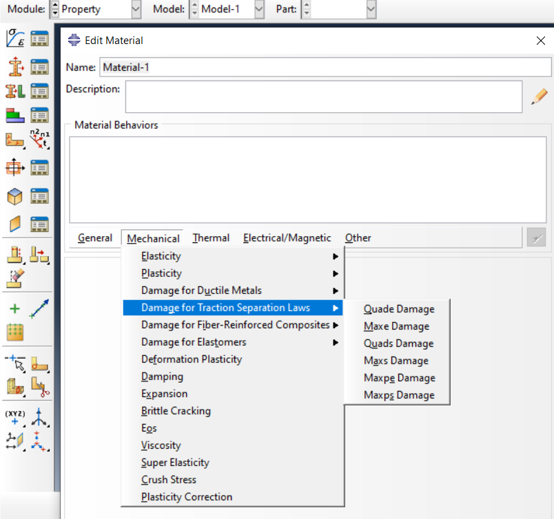
Figure 12: Traction-separation Abaqus built-in laws
4. Modified Compression Field Theory
The Modified Compression Field Theory (MCFT), developed by Vecchio and Collins in the 1980s, is a comprehensive model for analyzing the behavior of cracked reinforced concrete elements, especially under shear loading. It treats cracked concrete as a new orthotropic material, with unique stress-strain relationships that consider the effects of cracking, tension stiffening, and compression softening.
In MCFT, the stress-strain behavior of cracked concrete is characterized by average stresses and strains, accounting for the combined effects of local strains at cracks, strains between cracks, bond-slip, and crack slip.
Key Features:
- Captures the interaction between concrete and reinforcement in cracked regions.
- Suitable for analyzing shear-critical members.
Formulation:
- Compression Softening
Cracked concrete exhibits reduced compressive strength and stiffness due to transverse cracking. This phenomenon, known as compression softening, is modeled by reducing the compressive stress in the principal direction based on the transverse tensile strain.
The modified compressive stress ![]() is given by:
is given by:
Where:
 is the compression softening coefficient (function of transverse tensile strain)
 is the uniaxial compressive strength of concrete
 is principal compressive strain
 is the strain at peak compressive stress in uncracked concrete
-
- Tension Stiffening
After cracking, concrete can still carry tensile stress between cracks due to bond with reinforcement, a behavior termed tension stiffening. MCFT models this by defining a descending branch in the tensile stress-strain curve after cracking.
The tensile stress ![]() is given by:
is given by:
Where:
 is the tensile strength of concrete
 is the principal tensile strain
 is cracking strain
- n is the empirical parameter (typically between 0.5 and 1.0)
Get this post as a PDF file: caeassistant.com modeling-reinforcement-in-Abaqus
8. Conclusion
Simulating reinforced concrete in Abaqus is a key part of reliable concrete structure analysis. This guide showed how to model the interaction between concrete and steel using different techniques and failure models.
We started by explaining what reinforced concrete is and why it matters. Then, we looked at the basics of finite element analysis of reinforced concrete structures. You learned how to use rebar layers in shell or membrane elements, and how to apply the embedded region method in solid elements. Each method has its strengths depending on your model’s needs.
We also covered important failure models, including Concrete Damaged Plasticity (CDP), smeared and discrete crack models, and the Modified Compression Field Theory (MCFT). These tools help predict how reinforced concrete behaves under load, especially in complex or high-risk situations.
By using Abaqus concrete tools and applying the right methods, engineers can run accurate and efficient concrete simulations. This not only improves design quality—it helps create safer, more durable structures.
What is included in this package?
Workshops
Files
The topics in this package include, but are not limited to: concrete, beam-column structures, composites, steel rebars, Ultra-High-Performance-Fiber-Reinforcement Concrete columns, CFRP bars, etc.
Users ask these questions
In social media, users ask many questions regarding concrete simulation, reinforced concrete, etc. So, we decided to answer some of these questions, which you can see them below:
I. Stress of concrete exceeds the yield stress in tensile analysis
Q: The material properties of the rebar and concrete are set to be completely elasto-plastic. However, the yield stress is exceeded at the integration point of concrete.
The coefficient of friction is 0.3.
Why does the stress of concrete exceed the yield stress of material properties in the tensile analysis of rebar and concrete in Abaqus?
How can I prevent the yield stress from being exceeded?
Thank you in advance.
A: Hi,
I think it relates to your stress-strain curve. You see, when you want to define the Elastic/perfectly-plastic curve, you have to consider some rules. To avoid convergence problems, add a slight slope in the perfect plastic region (see the figure below).
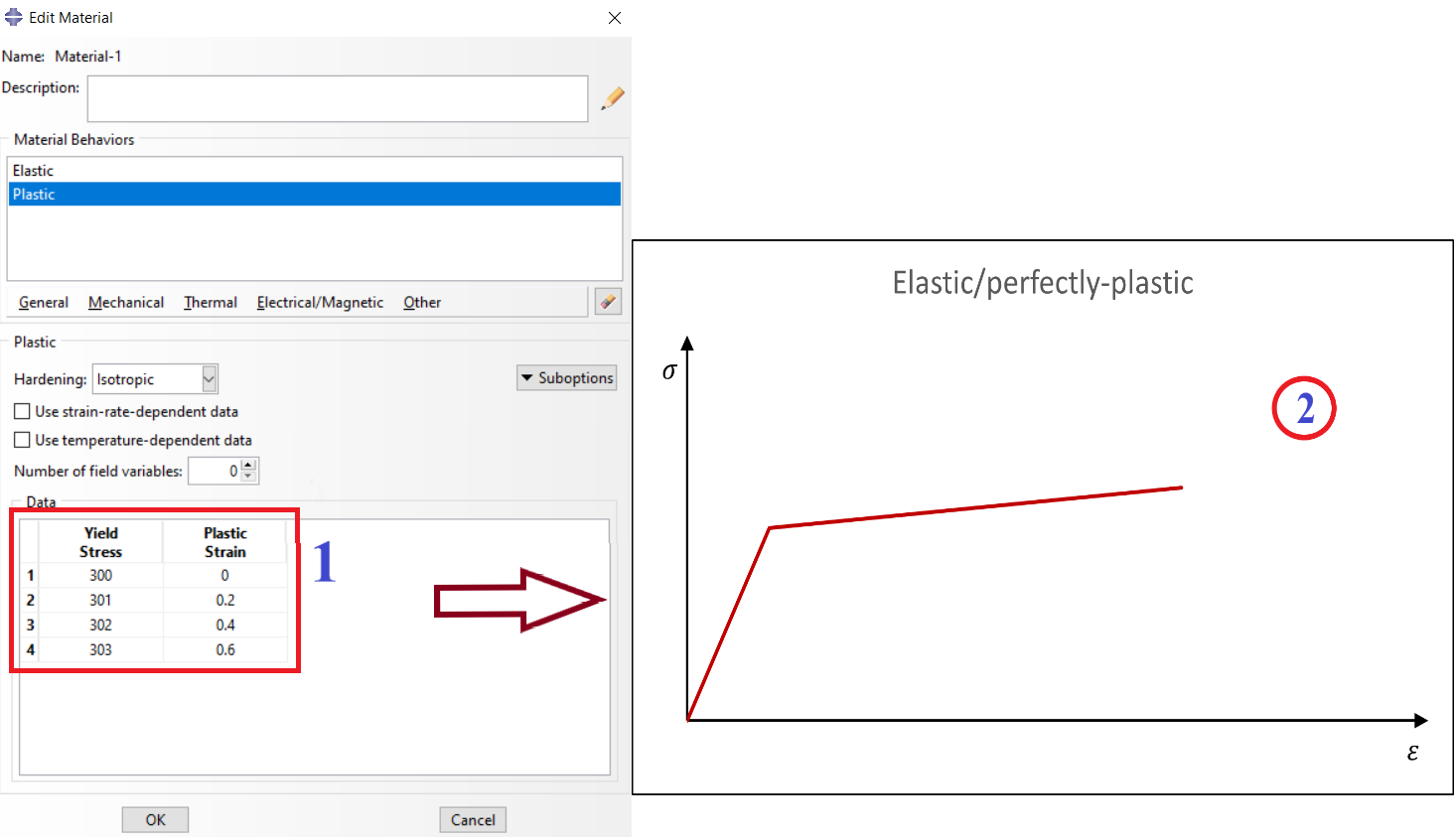
Note that all values in figure are just for example and don’t have to be true.
The CAE Assistant is committed to addressing all your CAE needs, and your feedback greatly assists us in achieving this goal. If you have any questions or encounter complications, please feel free to share it with us through our social media accounts including WhatsApp.
Explore our comprehensive Abaqus tutorial page, featuring free PDF guides and detailed videos for all skill levels. Discover both free and premium packages, along with essential information to master Abaqus efficiently. Start your journey with our Abaqus tutorial now!
wow, awesome blog post. Really thank you! Want more. Reeba Corbett Clapp
Hey, thanks for the article. Really looking forward to read more. Fantastic. Janice Darbee Leif
Hello friends, fastidious paragraph and good urging commented at this place, I am genuinely enjoying by these. Madelina Hendrik Loftis
I really like reading through a post that will make people think. Petrina Davis Gregorius
I was very pleased to find this web site. I want to to thank you for ones time just for this fantastic read!! I definitely enjoyed every bit of it and I have you saved as a favorite to check out new stuff in your blog. Di Moshe Rubio