
Ductile Damage: A Comprehensive Study on Failure Mechanisms of Ductile Materials
Ductile damage is a gradual degradation of a material’s strength caused by the accumulation of tiny microscopic defects. It plays a critical role in metals and alloys, which are widely used for their strength, durability, and ductility across industries like automotive, aerospace, and construction.
Understanding how ductile damage initiates, grows, and eventually leads to failure is essential for predicting the service life of components — and for designing materials that better resist cracking and breaking. Computational models have become powerful tools for simulating this complex process under different loading conditions.
In this blog, we’ll start from the basics — definitions, types of damage, and key concepts — before moving toward theories, practical applications, and finally, how ductile damage can be modeled effectively in Abaqus software.
1. What is Ductile Damage?
Have you ever pulled on a piece of aluminum foil and noticed how it stretches thinner before it finally tears? Even before you see any cracks, the inside of the material is already breaking down. That hidden process is a great example of ductile damage.
In simple words, ductile damage is the slow weakening of a material from the inside out. Tiny voids and cracks form inside the material as it undergoes plastic deformation — meaning it gets stretched or bent permanently, without snapping back.
Unlike brittle materials that shatter suddenly, ductile materials — like most metals — give plenty of warning. They stretch, bulge, and deform noticeably before they actually break. That’s why we trust metals for structures like bridges, cars, and airplanes — they don’t fail without giving a sign first.
In technical terms, ductile damage is about the accumulation and growth of microscopic voids within the material, leading to a gradual loss of strength and stiffness over time. Engineers need to understand this process to predict when structures might fail — and how to design them better.
Now that we’ve seen what ductile damage is, let’s dive deeper into the journey of how it actually happens inside a material…
2. The Stages of Ductile Failure
From micro-voids to complete material separation
Ductile failure doesn’t just happen in an instant. It’s a journey — a predictable and simulatable sequence of physical events that transforms a tough metal into a cracked remnant. Engineers divide this into three key stages:
2.1. Damage Initiation: When Trouble Begins
How does ductile damage start inside a material — and how do we model it?
At first, as you stretch a material past its elastic limit (where it can no longer return to its original shape), small defects start to appear inside.
Tiny voids, often around inclusions (tiny impurities) or second-phase particles, begin to form.
When a ductile metal is loaded, it doesn’t fail right away. But once the internal strain hits a certain threshold — especially under complex stress states — micro-voids begin to form. That’s when damage is said to initiate.
In simulation, we need a way to tell the software:
“Hey, start tracking damage now — the material has reached a critical point!”
This is where damage initiation criteria come in.
2.1.1. The Theory Behind It (Plastic strain Criterion)
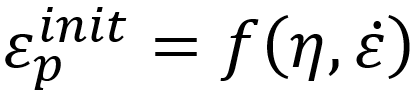
Many ductile damage models use a plastic strain criterion to define when damage starts.
In simple words, once the material’s equivalent plastic strain reaches a critical value, damage is considered initiated.
Ductile damage is often modeled based on accumulated plastic strain, influenced by two key factors:
-
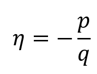
Stress triaxiality: Stress triaxiality is defined as the ratio of hydrostatic pressure pressure stress to the Mises equivalent stress.
-
Strain rate
 : how fast the material deforms.
These factors affect when voids nucleate and grow. So instead of using just one plastic strain value, we define the critical equivalent plastic strain as a function:
2.1.2. How It’s Set in Abaqus (Abaqus Ductile Damage)
In order to define this damage criterion (Abaqus ductile damage), you need to do as following:
“Property” Module> Create Material> Mechanical> Damage for Ductile Metals> Ductile Damage.
Then you need to provide the parameters shown in figure 1.
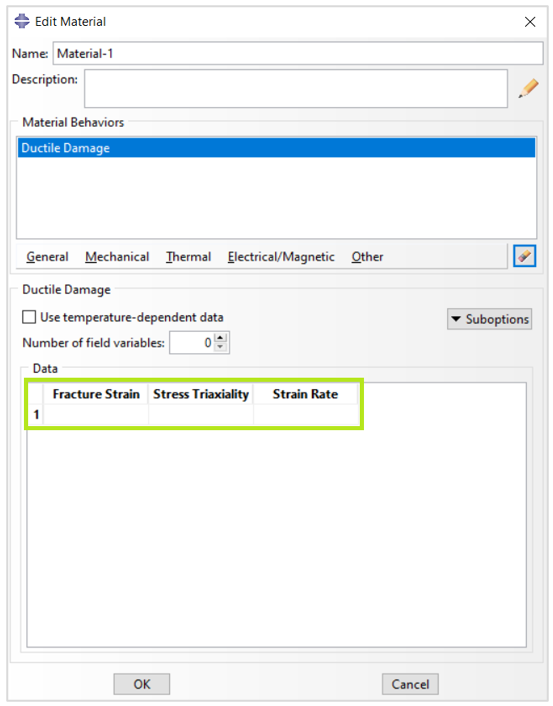
Figure 1: Defining Ductile damage in Abaqus
The parameters of ductile damages include:
- Fracture Strain (critical equivalent plastic strain): Equivalent fracture strain at damage initiation (
 )
) - Stress Triaxiality

- Strain Rate: The equivalent plastic strain rate ()
Abaqus interpolates between these points to determine when damage starts at each element in your mesh.
You can define:
-
Constant values (simpler),
-
Or a multi-point curve (more accurate and realistic).
📌 Pro Tip: If you’re unsure, start with a constant equivalent plastic strain (like 0.2 or 0.3) and build from there.
📏 Watch Your Units
The inputs are unit-sensitive:
-
Plastic strain: dimensionless
-
Strain rate: 1/s
-
Stress triaxiality: dimensionless
There are other damage initiation criteria which the Abaqus supports and you can see them in the picture below:
- Ductile
- Johnson-Cook
- Shear
- Forming Limit Diagram (FLD)
- Forming Limit Stress Diagram (FLSD)
- Marciniak-Kuczynski (M-K)
- Müschenborn-Sonne Forming Limit Diagram (MSFLD)
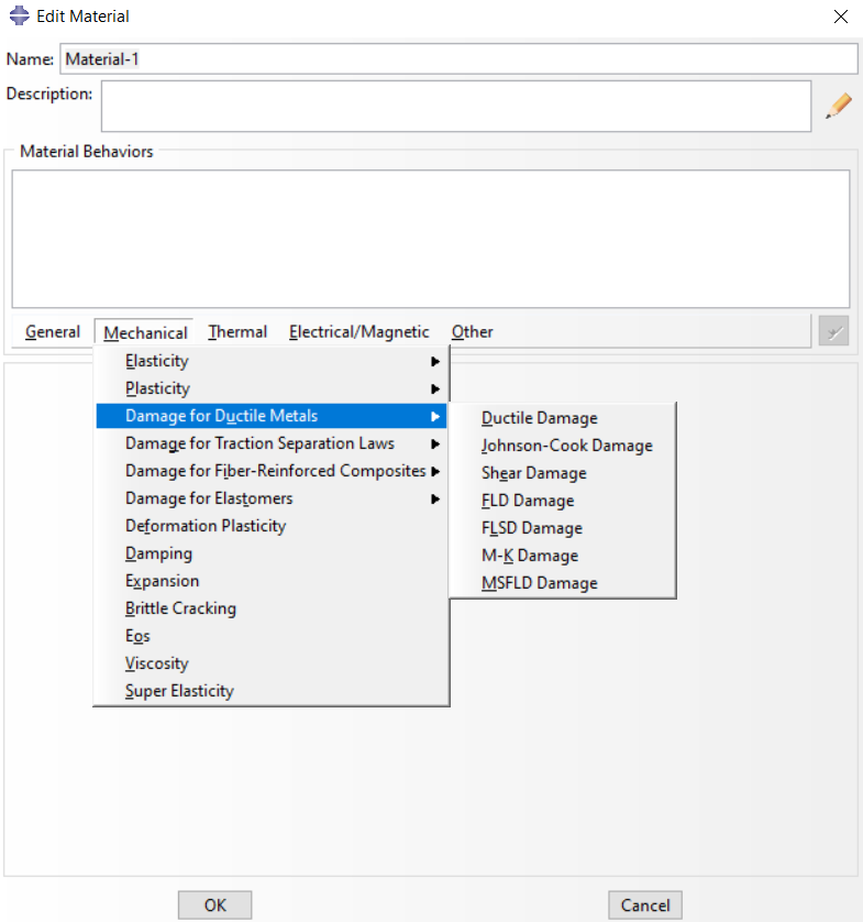
Figure 2: Defining ductile damage as material property in Abaqus/CAE
If you are interested we have a whole blog for one of the most popular criterion the Johnson Cook Model.
2.1.3. Shear damage criterion
The Shear damage initiation criterion is a model for predicting the onset of damage due to shear band localization. The model assumes that the equivalent plastic strain at the onset of damage is a function of the shear stress ratio and strain rate.
The shear stress ratio is defined as:
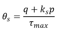
where q is the Mises equivalent stress, p is the pressure stress, and ![]() is the maximum shear stress and
is the maximum shear stress and ![]() is the material constant.
is the material constant.
To define this damage criterion, you need to do as following:
“Property” Module> Create Material> Mechanical> Damage for Ductile Metals> Shear Damage.
Then you need to provide the parameters shown in figure 3.
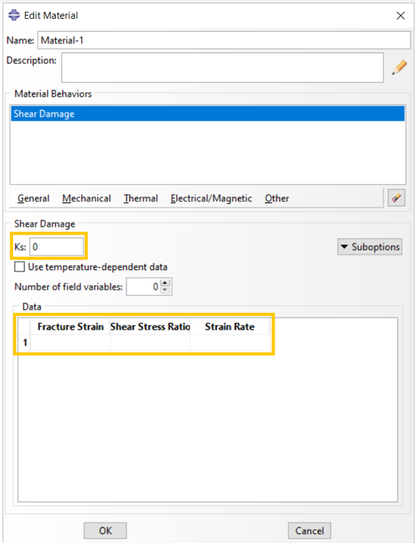
Figure 3: Defining Shear damage in Abaqus
The parameters of shear damages include:
- Fracture Strain (critical equivalent plastic strain): Equivalent fracture strain at damage initiation
- Shear Stress Ratio

- Strain Rate: The equivalent plastic strain rate
 or ()
or ()
An example of strain at damage initiation versus shear stress ratio diagram is shown in figure 4.
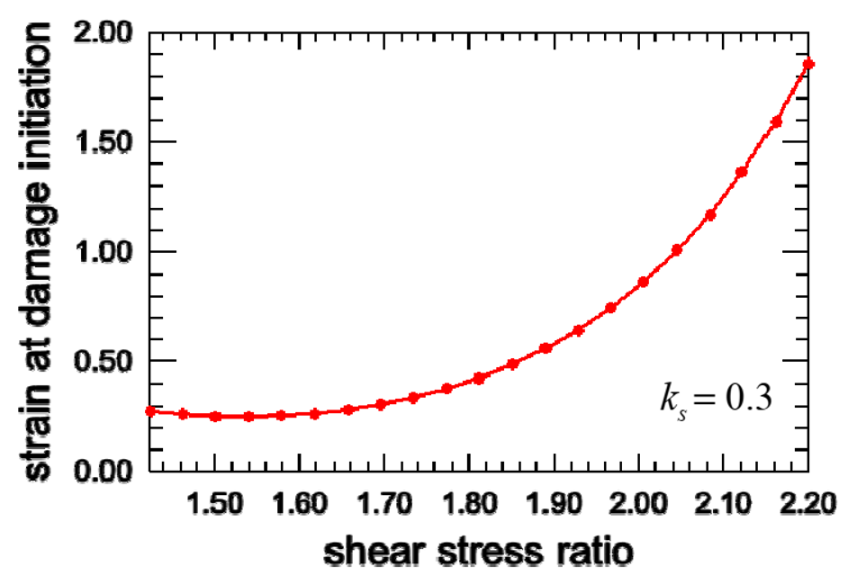
Figure 4: Shear criterion for Aluminum Alloy AA7108.50-T6 (Courtesy of BMW)
2.1.4. Forming Limit Diagram (FLD)
A forming limit diagram (FLD) is a plot of the forming limit strains in the space of principal (in-plane) logarithmic strains.
The FLD damage initiation criterion is intended to predict the onset of necking instability in sheet metal forming. The maximum strains that a sheet material can sustain prior to the onset of necking are referred to as the forming limit strains. Damage due to bending deformation cannot be evaluated using this model.
2.1.5. Forming Limit Stress Diagram (FLSD)
The FLSD damage initiation criterion is intended to predict the onset of necking instability in sheet metal forming. The strain-based forming limit curves (as used in the FLD criterion) are converted to stress-based curves to reduce the dependence on the strain path. This improves the performance of the FLSD damage model under conditions of arbitrary loading.
Similar to the FLD criterion, damage due to bending deformation cannot be evaluated using this model.
Forward Extrusion with discontinuous central bursts occurrence: This is one the examples in our full Ductile damage tutorial which is verified with research articles.
2.1.6. Marciniak-Kuczynski (M-K)
The M-K damage initiation criterion is used to predict sheet metal forming limits for arbitrary loading paths. The model introduces thickness imperfections, in the form of grooves, in the sheet material to simulate defects. Damage occurs when the ratio of deformation in the grooves relative to deformation in the original sheet thickness exceeds a critical value. By default, Abaqus evaluates four grooves at equally spaced angles of 0°, 45°, 90°, and 135° with respect to the local 1-direction of the material at each time increment and uses the worst result to determine damage initiation. The M-K criterion can be used in conjunction with the Mises and Johnson-Cook plasticity models, including kinematic hardening.
2.1.7. Müschenborn-Sonne Forming Limit Diagram (MSFLD)
The MSFLD damage initiation criterion is used to predict sheet metal forming limits for arbitrary loading paths. The model works based on equivalent plastic strain and assumes that the forming limit curve represents the sum of the highest attainable equivalent plastic strains. The approach requires transforming the original forming limit curve (without pre-deformation effects) from the space of major versus minor strains to the space of equivalent plastic strain, ![]() , versus the ratio of principal strain rates,
, versus the ratio of principal strain rates, ![]() .
.
Damage due to bending deformation cannot be evaluated using this model.
![]() So in summary, damage initiation is all about:
So in summary, damage initiation is all about:
-
Predicting the onset of failure,
-
Using physical parameters like plastic strain, triaxiality, and strain rate,
-
And feeding these into your FEA tool so it knows when to start tracking material degradation.
Once this is set up, you’re ready to move on to what happens after the damage begins — the evolution stage.
2.2. Damage Evolution: Growing Problems
So, damage has started… now what?
Once damage starts, the material begins to lose stiffness — gradually at first, then completely. This degradation is controlled by the damage evolution laws.
Damage evolution is how the material continues to lose stiffness and strength after the damage initiation threshold is reached. Think of it like this: once a crack forms, the surrounding area becomes weaker — and this weakness grows over time or under more load until the material completely fails.
2.2.1. Understanding the Theory Behind Damage Evolution

After damage begins in a ductile material, the degradation doesn’t happen all at once. Instead, it progresses — a process known as damage evolution. This progression depends on how much energy the material can absorb before it loses its ability to carry load.
This is where the damage energy release rate, Y, comes in. It essentially measures how much energy is being released as the material softens. The theory defines the damage evolution rate ![]() (i.e., how fast damage grows) as a function of Y.
(i.e., how fast damage grows) as a function of Y.
The damage energy release rate is given by:
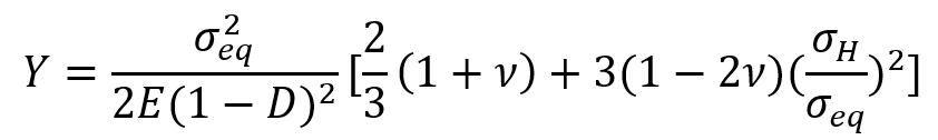
Where ![]() is the von Mises equivalent stress,
is the von Mises equivalent stress, ![]() is the hydrostatic stress,
is the hydrostatic stress, ![]() and
and ![]() are the Poisson’s ratio and the Young’s modulus of the undamaged material respectively.
are the Poisson’s ratio and the Young’s modulus of the undamaged material respectively.
![]() is the triaxiality ratio, which plays a very important role in the rupture of materials, the measured ductility at fracture decreases as it increases. Remember what is known from practice: “High triaxiality makes materials brittle!”
is the triaxiality ratio, which plays a very important role in the rupture of materials, the measured ductility at fracture decreases as it increases. Remember what is known from practice: “High triaxiality makes materials brittle!”
The evolution of the damage internal variable is assumed to be governed by the relation:
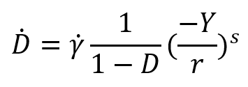
Where ![]() is the accumulated plastic strain, r, s are material constants.
is the accumulated plastic strain, r, s are material constants.
2.2.2. How Abaqus Implements Damage Evolution
The ductile damage criteria after initiation can follow the damage evolution by the parameters you define. They are all similar in this case. For example, for the ‘Ductile Damage’ to define the damage evolution, you need to do as follows:
“Property” Module> Create Material> Mechanical> Damage for Ductile Metals> Ductile Damage> Suboptions> Damage Evolution.
In the ‘Suboption Editor’ window, as shown in figure 5, you need to determine the parameters to define the damage evolution characteristics.
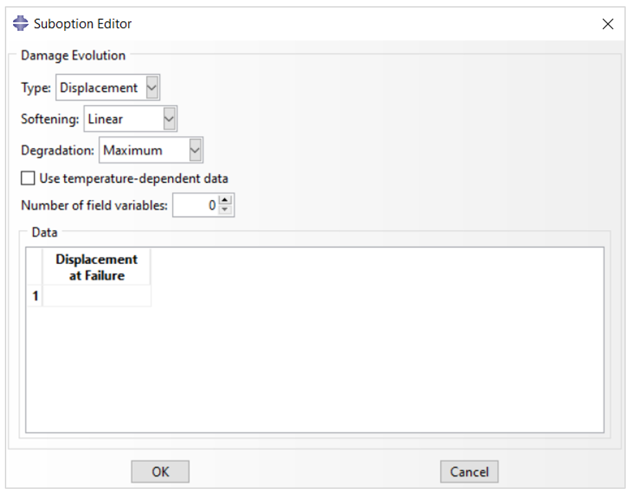
Figure 5: Determining damage evolution characteristics
The damage evolution parameters include:
- Type: This can be “Displacement” or “Energy”. We will explain these two later.
In the case of “Displacement” you need to enter the ‘Displacement at Failure’ and in the case of “Energy” you need to enter the ‘Fracture Energy’.
- Softening: This can be “Linear”, “Exponential” or “Tabular”.
The difference between these three models is shown in figure 6.
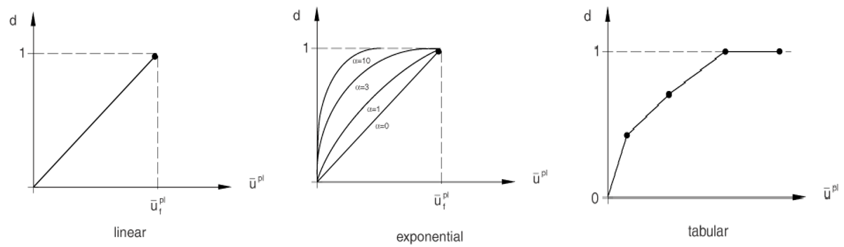
Figure 6: Different definitions of damage evolution based on plastic displacement
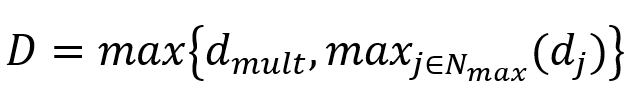
- Degradation: This can be “Multiplicative” or “Maximum”.
The overall damage variable, D, captures the combined effect of all active mechanisms and is computed in terms of individual damage variables, ![]() , for each mechanism. You can choose to combine some of the damage variables in a multiplicative sense to form an intermediate variable,
, for each mechanism. You can choose to combine some of the damage variables in a multiplicative sense to form an intermediate variable, ![]() , as follows:
, as follows:
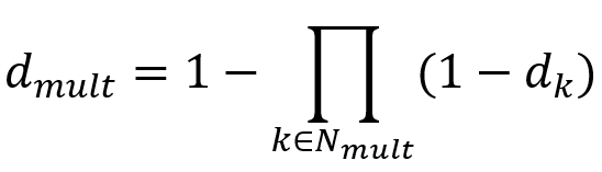
Then, the overall damage variable is computed as the maximum of ![]() and the remaining damage variables:
and the remaining damage variables:
In the above expressions ![]() and
and ![]() represent the sets of active mechanisms that contribute to the overall damage in a multiplicative and a maximum sense, respectively, with
represent the sets of active mechanisms that contribute to the overall damage in a multiplicative and a maximum sense, respectively, with ![]() .
.
You can also enter temperature if your model is temperature-dependent.
Now about the two types we have promised;
1. Displacement-Based Evolution
This method uses plastic displacement as the driver for damage progression. Think of it like saying, “After initiation, the material can stretch plastically by this much before it fails completely.”
Here, damage grows as a function of plastic displacement, not strain. Displacement isn’t mesh-sensitive, so this method is more stable across models.
When you use damage evolution based on effective plastic displacement in Abaqus, the effective plastic displacement is:

Where:
-
 : equivalent plastic strain,
 -
L: characteristic length of the element (automatically computed in Abaqus).
2. Energy-Based Evolution (Fracture Energy ![]() )
)
This approach is based on how much energy the material can absorb before failing after damage initiates. It’s the area under the stress-displacement curve from initiation to full failure:

Where:
-
: Fracture energy (J/m²)
-
 : Strain at damage start
 -
 : Strain at complete failure
You define ![]() in Abaqus, and it handles the rest.
in Abaqus, and it handles the rest.
-
Mesh-independent by default ✔️
-
Ideal when material toughness (energy to failure) is known
2.3. Final Failure: The Breaking Point
After damage initiation and evolution have done their part, we reach the grand finale — fracture. This is when the material loses its load-carrying capacity completely. Imagine a paperclip you’ve bent back and forth: at some point, it just snaps. That’s fracture.
What Happens at Fracture?
-
The stiffness of the material drops to zero.
-
The damage variable DD reaches 1.
-
The element is considered failed and is either deleted or no longer contributes to the structure.
In Abaqus, this is managed through element removal if specified. Once the damage variable hits a critical value, the element is taken out of the simulation.
3. Quick Recap on Ductile Damage
-
Initiation = Voids form (triggered by plastic strain).
-
Evolution = Voids grow and link up (damage grows based on displacement or energy).
-
Final Failure = Material can’t hold together anymore (fracture).
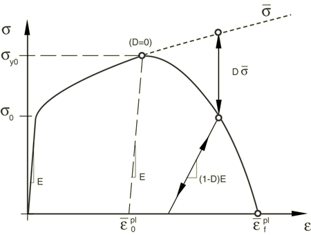
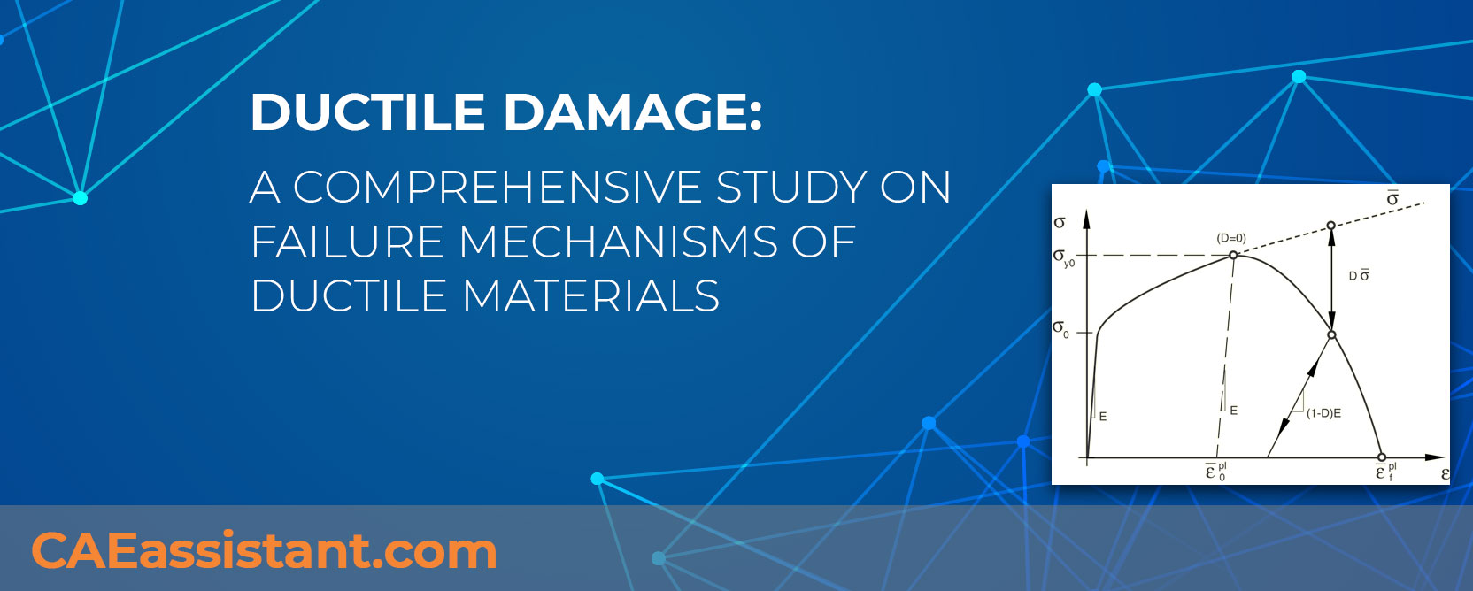
Figure 7: Stress-strain curve with progressive damage degradation
In figure 7, ![]() and
and ![]() are the yield stress and equivalent plastic strain at the onset of damage, and
are the yield stress and equivalent plastic strain at the onset of damage, and ![]() is the equivalent plastic strain at failure; that is when the overall damage variable reaches the value D=1.
is the equivalent plastic strain at failure; that is when the overall damage variable reaches the value D=1.
4. Ductile damage vs Brittle damage
The damage is called brittle when a crack is initiated at the mesoscale without a large amount of plastic strain. Just to give an order of magnitude, let us say that the ratio of plastic strain to elastic strain is below unity:
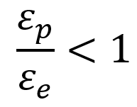
On the other hand, the damage is called ductile when it occurs simultaneously with plastic deformations larger than a certain threshold . It results from the nucleation of cavities due to decohesions between inclusions and the matrix followed by their growth and their coalescence through the phenomenon of plastic instability. Particularly damage models in ductile metals are proposed, and the Lemaitre model will be discussed.
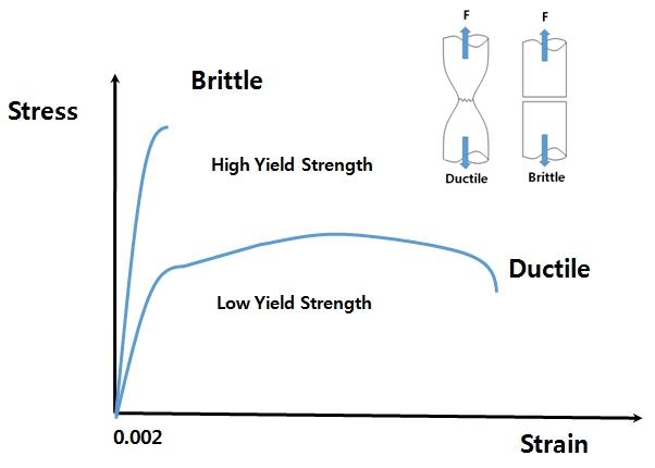
Figure 8: Ductile VS Brittle [Ref]
5. Popular Ductile Damage Models – The Brains Behind the Behavior
By now, we’ve walked through the stages of ductile failure: initiation, evolution, and fracture. We also explored how Abaqus implements these ideas.
But here’s an important point: those stages aren’t damage models themselves — they’re part of a framework for simulating how damage unfolds.
-
Initiation/evolution/fracture stages = Process of damage.
-
Damage models = Formulas and theories that describe how this process happens under specific conditions.
Think of the stages as the structure of a movie, and the models as the script and acting that give it emotion and depth.
Now let’s talk about the actual mathematical models that bring these stages to life.
1. Gurson–Tvergaard–Needleman (GTN) Model
-
Focus: Void nucleation, growth, and coalescence.
-
Highlights: Accounts for porosity, making it excellent for metals that fail due to micro-voids.
-
Used in: Many ductile fracture simulations, especially when voids dominate the failure mechanism.
Why it matters: GTN captures the entire damage progression within one model — no need to define initiation/evolution separately.
 If you want to know more about this theory and how to use it in FEA specially Abaqus, we have a complete tutorial of the GTN damage model.
2. Johnson–Cook Damage Model
-
Focus: High strain rate, thermal softening, and stress triaxiality.
-
Highlights: Includes parameters for strain rate and temperature, ideal for impact or explosion simulations.
-
Used in: Ballistics, crash tests, and anything with rapid deformation.
Why it matters: This model ties material response tightly to rate and heat — perfect for dynamic loading.
We have a complete article about this model all you want to know “Introduction to Abaqus Johnson-Cook Model: Accurately Model High-Strain rate Events“.
3. Lemaitre Model
-
Focus: Continuum damage mechanics (CDM).
-
Highlights: Treats damage as a scalar internal variable, modifying the stress-strain relationship.
-
Used in: Fatigue life predictions, low-cycle fatigue, or general CDM studies.
Why it matters: Lemaitre offers a smooth, gradual degradation, which is great for materials with no abrupt fracture.
There is a whole tutorial for this model as well “Ductile + Lemaitre (theory and Abaqus simulation)“
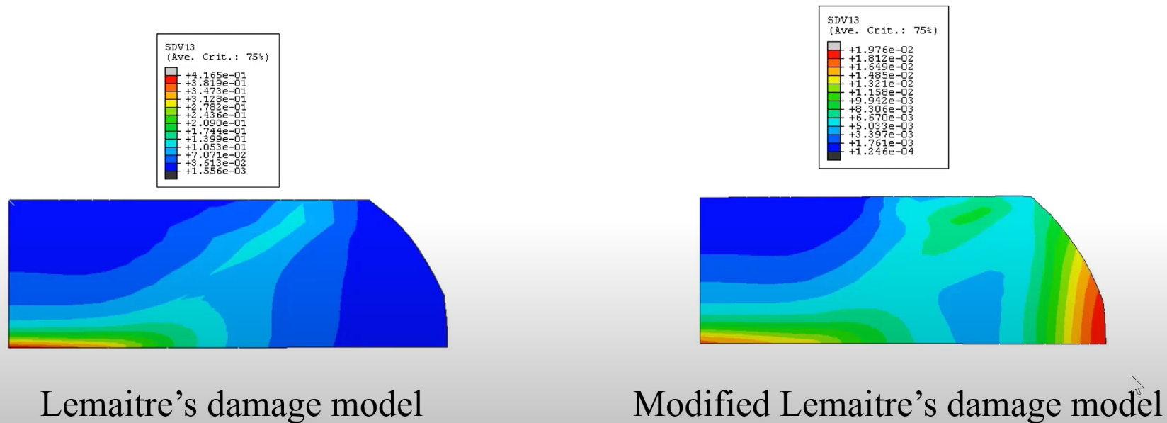
The example below shows you an Upsetting process simulation of a tapered specimen using Lemaitre damage model and modified Lemaitre which you can find its full tutorial and files in our Ductile damage full tutorial.
 |
 |
6. Practical Tips & Common Pitfalls in Ductile Damage Modeling
When it comes to modeling ductile damage, theory meets practice — and that’s where things can get tricky. While Abaqus provides powerful tools for simulating this complex behavior, accurate results depend on getting the details right. Here are some common pitfalls to watch out for, as well as practical tips on how to navigate them.
-
Accurate Material Parameters
-
Pitfall: Inaccurate values for damage-related parameters (like fracture strain and stress triaxiality) can throw off your simulation.
-
Tip: Spend time gathering experimental data or validated literature values, especially when working with new or custom materials.
-
-
Convergence Problems
-
Pitfall: Nonlinear simulations with ductile damage can encounter convergence issues, particularly in regions of high deformation.
-
Tip: Use Abaqus’s advanced solver settings, refine the mesh only where necessary, and ensure gradual load application to help your simulation converge.
-
-
Parameter Sensitivity
-
Pitfall: Simulation results can be extremely sensitive to the damage parameters you choose. Small changes might lead to large differences in predicted behavior.
-
Tip: Calibrate your model carefully with experimental data and perform sensitivity analyses. This helps you understand how parameters affect your results and guides you in choosing robust values.
-
Remember, overcoming these challenges is all about combining good experimental data, a solid understanding of material behavior, and utilizing the powerful solver settings available in your simulation tool.
 Recap
Recap
Now that we’ve covered some common pitfalls, let’s wrap up with a few general best practices to ensure a smooth modeling experience:
-
Start simple: Begin with a simple model and then progressively add complexity (e.g., more realistic material behavior or finer meshes) once you understand how the model behaves.
-
Use damage initiation and evolution separately: Keep the initiation and evolution steps clearly defined and independent of each other to avoid confusion.
-
Check mesh independence: Always perform a mesh convergence study to make sure that your results are not heavily influenced by mesh size.
| Pitfall | Solution |
|---|---|
| Inaccurate Material Parameters | Calibrate using experimental data, focus on key parameters |
| Convergence Issues | Refine the mesh, use advanced solver settings like stabilization |
| Sensitivity to Damage Parameters | Perform sensitivity analysis, calibrate with experimental data |
| Complexity & Computation Overhead | Start with simpler models and gradually increase complexity |
7. What is Damage in mechanical engineering?
The damage of materials is the progressive physical process by which they break. All materials are composed of atoms, which are held together by bonds resulting
from the interaction of electromagnetic fields. When debonding occurs, this is the beginning of the damage process.
At the microscale level, this is the accumulation of micro stresses in the neighborhood
of defects or interfaces and the breaking of bonds, which both damage the material.
At the mesoscale level of the representative volume element (RVE), this is the growth and the coalescence of microcracks or microvoids which together initiate one crack.
At the macroscale level, this is the growth of that crack. The two first stages may be studied using damage variables of the mechanics of continuous media defined at the mesoscale level. The third stage is usually studied using fracture mechanics with variables defined at the macroscale level.
You may wonder what are these scales? Let’s define them from the smallest to the biggest.
- The microscale is the scale of the mechanisms used to consider strains and damage.
- The mesoscale is the scale at which the constitutive equations for mechanics analysis are written.
- The macroscale is the scale of engineering structures.
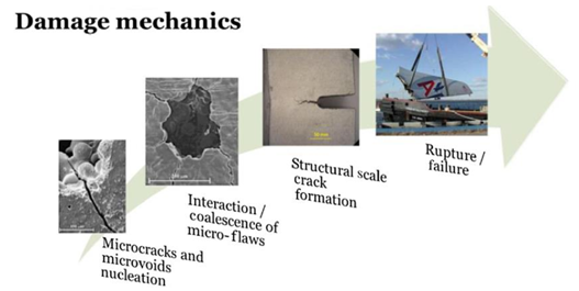
Figure 1: Damage progressive process
1.2. Mechanical Representation of Damage
Consideration of the simple one-dimensional case of a homogeneous damage pictured in Figure 2 leads to the simple definition of damage as the effective surface density of microdefects:
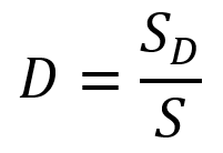
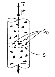
Figure 2: One-dimensional damaged sample under tension
S in this equation is the surfaces free of microcracks or microcavities and ![]() is the surface of microcracks or microcavities. It is convenient to introduce an effective stress
is the surface of microcracks or microcavities. It is convenient to introduce an effective stress ![]() related to the surface that effectively resists the load, namely
related to the surface that effectively resists the load, namely ![]() :
:
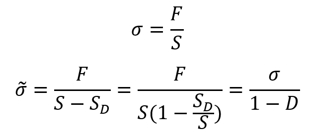
This definition is the effective stress on the material in tension. In compression, if some defects close, the damage remaining unchanged, the surface that effectively resists the load is larger than ![]() . In particular, if all the defects close, the effective stress in compression is equal to the usual stress
. In particular, if all the defects close, the effective stress in compression is equal to the usual stress ![]() .
.
Lemaitre stated the ‘Strain Equivalent Principle’ for damage which says:
“Any strain constitutive equation for a damaged material may be derived in the same way as for a virgin material except that the usual stress is replaced by the effective stress”.
Is it complicated? Let’s say it in a simpler way.
Consider an undamaged material for which D = 0. Assume a constitutive equation for this material which is the relation between strain and stress like:
Now consider a damaged material for which ![]() . The Strain Equivalence Principle says that the constitutive equation remains unchanged but instead of
. The Strain Equivalence Principle says that the constitutive equation remains unchanged but instead of ![]() you must use
you must use ![]() in this equation.
in this equation.
A schematic of this statement is shown in figure 3.
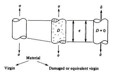
Figure 3: Schematic of Strain Equivalent Principle
8. How to write a Ductile Damage VUMAT?
Modeling ductile damage in Abaqus VUMAT requires a constitutive model that accurately describes the damage evolution process. This section describes an algorithm for the implementation of the elastic-plastic-damage constitutive equations including the effect of crack closure. Algorithms based on the operator split concept, resulting in the standard elastic predictor/plastic corrector format, are widely used in computational plasticity. The flow chart of the elastic predictor/return mapping algorithm for the elastic-plastic-damage model is implemented as shown in figure 8 based on the article titled “Numerical analysis of damage evolution in ductile solids”.
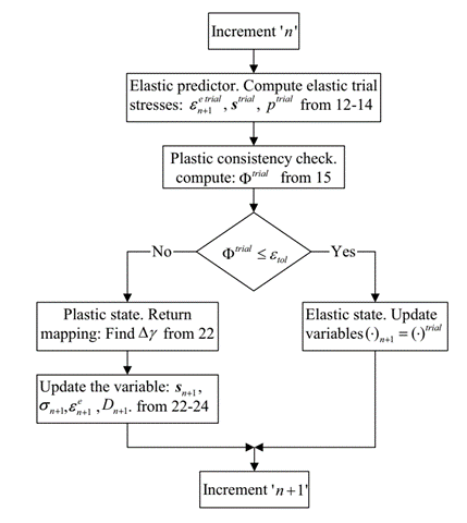
Figure 18: Flow chart of elastic predictor/return mapping algorithm for the elastic-plastic-damage model
8.1. Ductile Damage VUMAT Subroutine
To introduce the ductile damage Abaqus model, a user material subroutine VUMAT is developed in the Abaqus software package. In the VUMAT subroutine, the damage variable will be calculated in each of the integration points (or Gauss points) locally. The element deletion option is used with VUMAT to induce ductile crack growth. The developed VUMAT subroutine has the ability to analyze ductile damage in three-dimensional and plane strain cases. 3D and 2D plane strain problems. The VUMAT subroutine is run in the Abaqus/Explicit, it can be used in various problems that require complex contact algorithms.
Using VUMAT to implement ductile damage models offers several advantages:
- Customization
Allows for the incorporation of complex damage mechanisms and user-defined material behavior.
- Versatility
Applicable to a wide range of engineering problems and materials.
- Accuracy
Provides a precise representation of damage evolution, leading to more reliable FEA results.
In order to get access to the ductile damage VUMAT subroutine in Abaqus you can see the following link:
“Ductile Damage Abaqus model for 3D continuum element (VUMAT Subroutine)“
Now let’s check how accurate and reliable our VUMAT is.
8.2. Ductile Damage VUMAT Verification
Calibrating and validating the ductile damage model implemented in VUMAT is crucial for obtaining reliable FEA results. This involves comparing the numerical predictions with experimental or physical test data.
For verification of the VUMAT, the simulation of a three-point bending test is investigated (Figure 19).
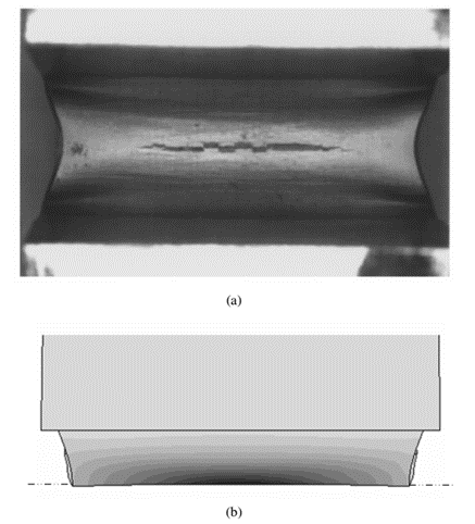
Figure 19: Comparison of experimental Giovanola et al. (1999) crack initiation site in three-point bending test with
Figure 19 (a) shows the real three-point bending test and as you can see the crack is propagated from the middle of the sample. Figure 19 (b) also shows the damage contour provided by the ductile damage VUMAT. The result is earlier damage localization and deterioration of the central region compared to the outer edges. This suggests that fracture initiation should be expected in this region. This result is in agreement with the experimental observations.
8.3. Ductile Damage VUMAT Application
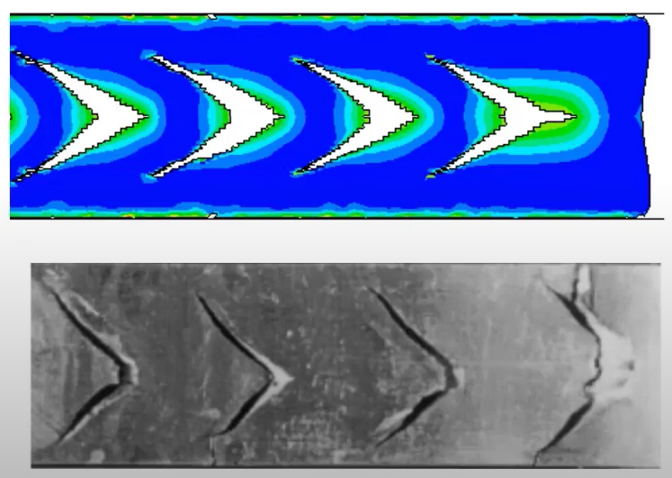
After the VUMAT subroutine is verified, it can be used to predict the occurrence of damage growth and failure in various mechanical processes. For example; the modified ductile damage model is applied to predict the initiation of the micro-void as a central burst along the bar axis during the forward extrusion (Figure 20).
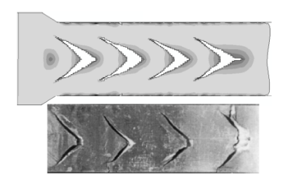
Figure 20: Prediction of central burst along the bar axis during the forward extrusion
This tutorial package starts with the fundamentals of ductile damage and damage mechanics, then takes you deep into the Lemaitre Damage Model—covering its theory, limitations, and a modified approach. You’ll also learn how to implement it in ABAQUS using VUMAT. To top it off, 3 practical examples are included, with results benchmarked against published research, making this a powerful resource for engineers and researchers aiming for accurate, research-level simulations.
 |
|
9. Final Thoughts
Modeling ductile damage isn’t just about plugging numbers into software — it’s about understanding how materials behave, why they fail, and how we can simulate that failure with confidence.
Throughout this guide, we’ve gone from the basic concepts of ductile failure to the more advanced theories and practical steps needed for implementation. We’ve explored initiation, evolution, and the models behind them — all while keeping things grounded and actionable.
Remember:
-
The theory comes first — tools like Abaqus are only as good as the models and parameters you feed them.
-
Mesh size, material data, and solver settings can make or break your simulation.
-
Validation isn’t optional — always compare with experimental data when possible.
Whether you’re designing safer automotive components, testing new alloys, or optimizing manufacturing processes, a strong grasp of ductile damage modeling will set you apart.
Stay curious, test rigorously, and never stop asking “Does this reflect reality?”