
Fatigue Analysis Introduction | Abaqus Fatigue, Fatigue Life Prediction, Cyclic Loading Types

Fatigue damage is a common yet complex phenomenon in materials exposed to repeated or cyclic loads. Over time, even under stress levels well below a material’s breaking point, cracks may develop and grow, eventually leading to failure. But how to predict the occurrence of this phenomenon? Understanding how fatigue affects different materials is crucial for industries ranging from aerospace to automotive, where structural integrity is paramount.
In materials like metals, polymers, and composites, fatigue damage unfolds in stages—starting with crack initiation, followed by crack growth, and culminating in final fracture. Engineers use various models and analysis tools to predict how long a material can withstand cyclic loading before failing. This article explores different types of cyclic loading patterns and explains how fatigue evolves. If you’re planning to perform a fatigue analysis using Abaqus, it’s essential to have knowledge about the loading conditions, material fatigue properties, and the type of fatigue (low-cycle or high-cycle) you want to simulate.
This article takes a comprehensive look at fatigue from multiple angles. It begins by defining the concept of fatigue damage and provides real-world examples from different industries, such as bridge collapse, and rotating machinery failure. We also explore the types of cyclic loading patterns that lead to fatigue, including fully reversed and asymmetric loading. Further sections dive into the stages of fatigue crack growth, the critical Paris Law for crack propagation, and fatigue life prediction using S-N curves. You’ll also learn how to perform fatigue simulations in Abaqus, from setting up the model to analyzing fatigue behavior using S-N curves and strain-life methods.


1. What is Fatigue Damage and Fatigue Analysis?
Fatigue failure can occur in three main stages:
- Crack initiation: Small imperfections or stress concentrations (like surface roughness, voids, or notches) begin to develop into micro-cracks after repetitive loading.
- Crack propagation: These micro-cracks expand with each loading cycle, growing slowly across the material’s surface or internally.
- Final fracture: Once the cracks reach a critical size, the material can no longer withstand the stress, leading to sudden and often catastrophic failure.
The process of fatigue is complex because it depends on various factors such as load amplitude, mean stress, material properties, surface conditions, and environmental influences (e.g., corrosion). Fatigue can occur in metals, polymers, ceramics, and composites (Composite Fatigue) under cyclic loading conditions. Let’s examine some real examples of the fatigue phenomenon.
1.1. Real examples of Fatigue | Fatigue Analysis Example
- Shoes: Over time, the soles of shoes wear down due to the repetitive compressive and tensile forces experienced during walking or running. The materials used in shoes undergo fatigue, which leads to degradation and eventual failure.
- Bridges: Bridges experience cyclic loading from vehicles passing over them. The repeated stresses can cause fatigue cracks in the steel or concrete structure. For example, a bridge in the United States, the Silver Bridge collapse in 1967 was attributed to the fatigue of an eyebar, a critical load-bearing component of the bridge. This was another fatigue analysis example to understand why fatigue analysis is important.
- Rotating Machinery: Components like turbine blades, gears, and axles experience cyclic stresses during their operation. Over time, these stresses can cause fatigue cracks. The failure of a turbine blade due to fatigue in jet engines can lead to catastrophic engine failure.
Fatigue is crucial in engineering design because it can lead to unexpected failures if not properly accounted for. Designers must predict the fatigue life of a component and ensure it can withstand the expected number of load cycles throughout its operational life. This is especially important for structures or components subjected to repeated or fluctuating stresses. In the next sections, we will examine the important issues of the fatigue phenomenon together.
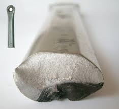
Figure 1: Failure of a crank arm due to fatigue
 |
Abaqus Fatigue tutorial Examples:
|
2. Types of Fatigue Loading (Cyclic Loading)
Fatigue damage is caused by cyclic loading, where repeated or fluctuating stresses act on a material over time. There are several types of cyclic loading patterns that contribute to fatigue analysis. Each type can have different effects on the material, leading to various fatigue failure behaviors. The most common cyclic loading types that can lead to fatigue are:
2.1. Fully Reversed Cyclic Loading
In fully reversed cyclic loading, the stress alternates between positive (tensile) and negative (compressive) stress. The magnitude of tension and compression is equal. Here is stress-time diagram:
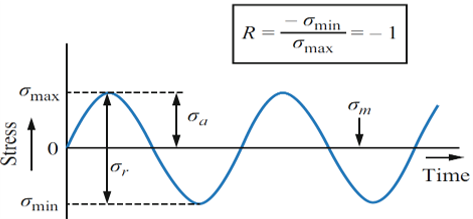
Figure 2: Fully Reversed Cyclic Loading stress-time curve
For example, Crankshafts in internal combustion engines are subjected to fully reversed cyclic loading as they rotate, alternating between tension and compression with each revolution.
To calculate the mean stress, stress amplitude, and stress range, the following equations, respectively labeled as 1 to 3, are used:
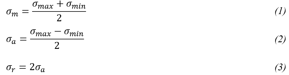
2.2. Asymmetric Cyclic Loading
Asymmetric cyclic loading has stresses that do not alternate equally between tension and compression. The minimum stress is greater than zero (it never reaches the compressive range), and the mean stress is not zero. This type of loading is common in many real-world applications where loads fluctuate but don’t reverse entirely.
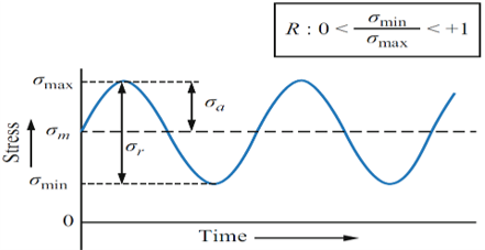
Figure 3: Asymmetric Cyclic Loading stress-time curve (The minimum stress is greater than zero)
If the minimum stress is less than zero (reaches the compressive range) and the average stress is not zero, the loading is the asymmetric cyclic loading type.
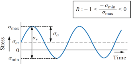
Figure 4: Asymmetric Cyclic Loading stress-time curve (minimum stress is less than zero)
2.3. Repeated Cyclic Loading
In repeated cyclic loading, the stress oscillates between a maximum positive stress and a zero or minimum positive stress. The stress does not alternate to negative values (compression), meaning the material is primarily under tension.
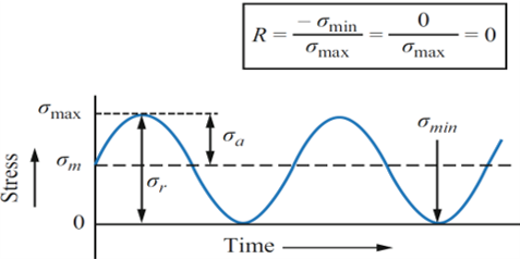
Figure 5: Repeated Cyclic Loading stress-time curve
2.4. Random Cyclic Loading
In random cyclic loading, the stress varies in an unpredictable manner with both amplitude and frequency fluctuating randomly. It often occurs in components subjected to varying loads with no fixed pattern, making fatigue prediction more challenging. For example, wind turbine blades undergo random cyclic loading due to the variable nature of wind speeds and directions. These random loads cause stresses on the blades, leading to fatigue over time.
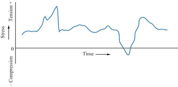
Figure 6: Random Cyclic Loading stress-time curve
3. Fatigue Analysis Crack Growth
The fatigue process consists of several stages that describe how damage accumulates in a material due to cyclic loading. Understanding these stages is critical for predicting in fatigue analysis when a component will fail due to fatigue.
As we explained before, crack initiation is the first stage of the fatigue process, where micro-cracks form in the material. Crack initiation usually occurs in areas of high-stress concentration, such as surface defects, inclusions, or sharp notches. The cyclic loading leads to microscopic defects like grain boundary separations. After crack initiation, the crack begins to grow with each loading cycle. The rate at which the crack grows depends on the material properties, the applied load, and the environment. In this stage, the crack propagates incrementally with each stress cycle, and the size of the crack increases, leading to a reduction in the material’s load-carrying capacity.
As the crack grows, it passes through three different phases based on the rate of crack growth:
You can find tutorial videos for 2D and 3D Fatigue crack growth simulations along with simulation files (inp, odb, etc) in the package below.

3.1. Threshold Region
In this region, the stress intensity factor range ΔK is very low, and the crack growth rate is negligible. There is a threshold value of ΔK called ΔKth below which no crack growth occurs. The stress intensity factor range (ΔK) is introduced by the equation below.
![]()
Where:
 is the cyclic stress range.
 is the crack length.
 is a constant.
3.2. Stable Crack Growth Region
In this region, the crack growth rate follows a steady, predictable pattern. The rate of crack propagation is typically proportional to a Paris Law. This is the most important region for engineers because most of the component’s life is spent in this stage.
3.3. Rapid Fracture Region
As the crack reaches a critical size, the stress intensity factor increases rapidly, and the crack propagation rate accelerates. The crack grows uncontrollably until the material fractures.
3.3.1. Paris Law: A Crack Growth Theory
One of the most widely used theories for predicting fatigue crack growth is Paris Law, which describes the relationship between the crack growth rate and the applied cyclic stress intensity factor. It is applicable in the second region of the crack growth process, where the crack growth rate is stable. Paris Law is given by the following equation:
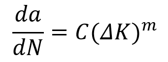
Where:
 is the crack growth rate (i.e., the crack extension per load cycle).
 is the stress intensity factor range, which represents the difference between the maximum and minimum stress intensity factors during a loading cycle.
- C and m are material constants that are determined experimentally. They depend on the material and the environment.
As the crack length “![]() ” increases, the stress intensity factor range (ΔK) increases, leading to faster crack growth. Paris Law helps in predicting how fast a crack will grow under given cyclic loads and when it will reach a critical size, causing failure.
” increases, the stress intensity factor range (ΔK) increases, leading to faster crack growth. Paris Law helps in predicting how fast a crack will grow under given cyclic loads and when it will reach a critical size, causing failure.
Using Paris Law, engineers can predict the number of cycles a component can endure before failure. By integrating the Paris Law equation, the remaining fatigue life can be calculated based on the initial crack size ![]() , the final critical crack size
, the final critical crack size ![]() , and the material constants C and m.
, and the material constants C and m.
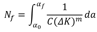
Where:
- Nf is the number of cycles to failure.
 is the initial crack size.
 is the critical crack size.
This equation allows for the prediction of when a crack will grow to a dangerous size and enables engineers to design maintenance schedules or preventive measures accordingly.
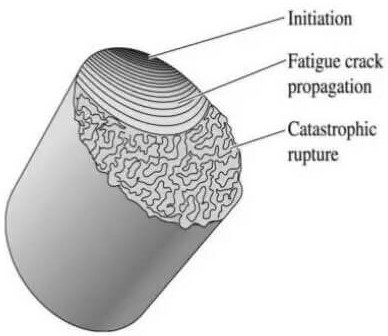
Figure 7: Typical fatigue fracture surface
4. Fatigue Cycle Number
Fatigue cycle number refers to the number of load cycles a material can endure before a fatigue crack leads to failure. It is a crucial concept in fatigue analysis and helps determine the lifetime of components subjected to cyclic loading. Fatigue life is typically expressed as the total number of cycles a material can withstand before failure, denoted by N.
The fatigue life of a material is categorized based on the number of cycles to failure. These categories help to distinguish between different types of fatigue behavior, which vary depending on the magnitude of applied stress, material properties, and environmental conditions.
4.1. Low-Cycle Fatigue (LCF)
Low-cycle fatigue occurs when the material experiences high cyclic stresses, which induce significant plastic deformation in each cycle. The material undergoes fewer load cycles before failure in this kind of fatigue analysis(typically fewer than 10,000 cycles).
4.2. High-Cycle Fatigue (HCF)
High-cycle fatigue occurs when the material is subjected to lower stress levels, typically within the elastic range. The cyclic stresses are lower, meaning the material can endure a large number of load cycles before failure. For this type of fatigue, lifetime is typically in the range of 10,000 to 1,000,000 cycles or more.
There are also two other types of fatigue analysis known as Very High-Cycle Fatigue (VHCF) and Very Low-Cycle Fatigue (VLCF). In Very High-Cycle Fatigue, due to the very low stress level, the number of cycles can reach over one billion cycles (10⁹ cycles), but Very Low-Cycle Fatigue is an extreme form of low-cycle fatigue where very few cycles (often fewer than 10) are required to initiate and propagate cracks. These types of fatigue occur less frequently.
5. Fatigue Life (S-N curve) | Fatigue Life Prediction
- Fatigue Life
Fatigue life is the total number of stress cycles a material can endure before failure occurs due to fatigue. It represents the lifetime of a component under repeated cyclic loading. Fatigue life is often denoted as N, which refers to the number of cycles to failure. Fatigue life prediction is crucial for ensuring the long-term durability and safety of components subjected to cyclic stresses, especially in fields like aerospace, automotive, and civil engineering.
- Fatigue Life Curve (S-N Curve)
The S-N curve is a graphical representation that shows the relationship between the stress amplitude (S) and the number of cycles to failure (N). It is widely used to predict fatigue life under constant amplitude loading. The S-N curve is typically plotted on a logarithmic scale, with stress amplitude on the vertical axis and the number of cycles to failure on the horizontal axis.
Some materials, particularly ferrous metals (such as steel), exhibit an endurance limit. This is the stress amplitude (Se) below which the material can theoretically endure an infinite number of cycles without failing.
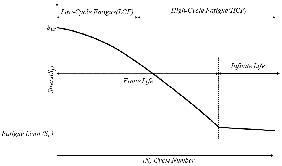
Figure 8: Fatigue life curve (S-N curve)
5. How to do an Abaqus Fatigue Analysis?
Abaqus is a very powerful software that provides its users with the ability to simulate fatigue. One of the features of Abaqus that is used for fatigue simulation is “Direct Cyclic” analysis. To better understand the performance of Abaqus in fatigue simulation, it is better to first examine this direct cyclic analysis.
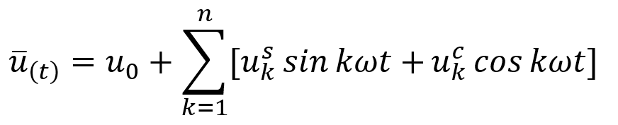
The elastic-plastic behavior of parts under cyclic load goes to a stable state after a certain number of cycles and the stress-strain relationship of the material does not change. The classical methods for obtaining the number of cycles at which the behavior of the part becomes stable have been to apply a cyclic load to the part over time until the behavior of the part becomes stable. The problem with this method is that it is time-consuming to perform the analysis in a high number of cycles. To solve this problem, the “Direct Cyclic” analysis method has been presented in the Abaqus software, in which a displacement function is defined for all analysis times as a Fourier series.
In this relation, n is the number of cycles, T is the time period, ω is the frequency, and u is the constants that must be calculated. In the Abaqus software, this equation is solved by Newton’s method and the amount of stable cycle displacement of the part is calculated at all times.
In the First example of this tutorial (2D Fatigue crack growth), you will learn:
Low-cycle fatigue analysis
The previous methods for fatigue analysis are based on the S-N diagram (force versus number of cycles to failure), which is still used in many engineering designs. This method models the overall behavior of the part and does not provide a relationship between the number of cycles and damage to the part or the length of the cracks in the part.
An alternative method is to predict fatigue life using crack and failure laws based on inelastic strain/energy in the stable cycle of the part. Since modeling the failure behavior and crack formation under high-number loading cycles is very time-consuming, it is possible to examine the behavior of the part at low cycle numbers and predict the crack length and its distribution under high cycles using experimental relations.
To calculate the fatigue life of parts in Abaqus software, the “Direct cyclic” analysis method is combined with the continuum damage mechanics method or the linear elastic fracture mechanics method, and its life is predicted based on the crack growth in the part.
First, the behavior of the part under different load values and a different number of cycles is calculated, and these results are used to predict the material properties at each increment, which is equivalent to a certain number of loading cycles. The results of each increment are used as the initial value in the next increment, so the crack length is updated at each increment. The applied load is gradually increased until the fatigue load of the part is calculated.
5.1. Continuum Damage Mechanics (CDM) Method
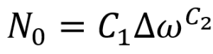
The first method is based on continuum damage mechanics, which is suitable for ductile materials. In this method, cyclic loads cause plastic strain accumulation and ultimately cause cracks to form and propagate in the part. The number of cycles after which a crack will form (![]() ) is predicted in this method based on the amount of hysteresis strain energy (
) is predicted in this method based on the amount of hysteresis strain energy (![]() ) per cycle. The relationship between the amount of hysteresis strain energy per cycle and the final number of cycles that the part will withstand is given below, where
) per cycle. The relationship between the amount of hysteresis strain energy per cycle and the final number of cycles that the part will withstand is given below, where ![]() and
and ![]() are material constants that must be defined.
are material constants that must be defined.
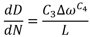
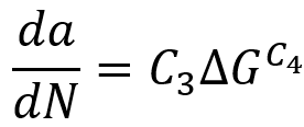
When a failure initiation occurs in a part of the part, the post-failure behavior of the part is modeled through the failure rate in terms of the number of cycles according to the following equation, where C3 and C4 are material constants that must be defined. L is known as the integration length, which is different for different elements. In the first-degree three-dimensional and plane elements, the length of the element diameter is considered, and in the second-degree element, the half-diameter of the element. In beam elements, the length of the element is considered, and in cohesive elements, the thickness of the element is considered.
These two parameters, namely hysteresis strain energy and failure rate, are used in fatigue simulation as criteria for crack initiation and crack progression.
As explained, direct cyclic step can be used to simulate fatigue. This step uses Fourier series and the number of Fourier series iterations per increment is adjustable.
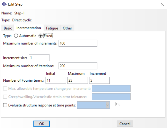
Figure 10: Direct cyclic step, Incrementation tab
Also, to perform fatigue analysis, the Low Cycle Fatigue option must be enabled. In this tab, you can also specify the number of cycles for analysis. The Damage value is extrapolated at each increment through the following equation. In Abaqus software, it is possible to enter the minimum and maximum number of cycles that are extrapolated from the following equation, which can be set. The default values for the minimum and maximum are 100 and 1000, respectively.

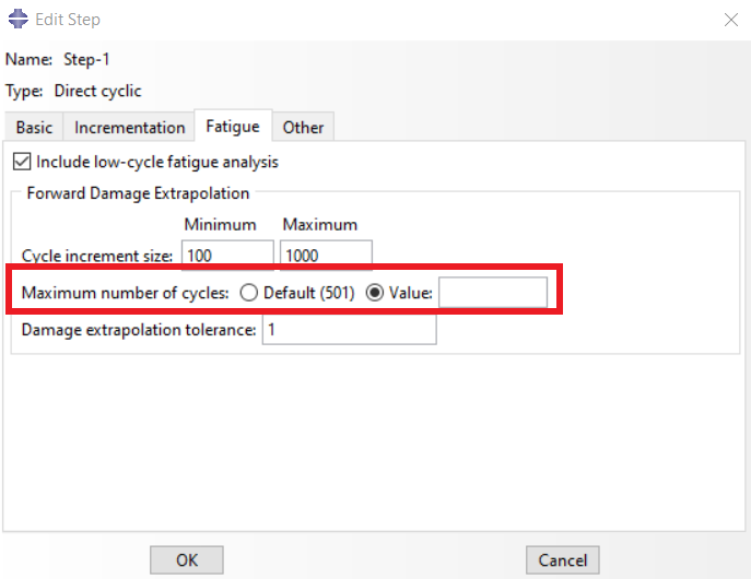
Figure 11: Direct cyclic step, Fatigue tab
Another important point in fatigue simulation using this method is to use the appropriate amplitude. In loading, we should use the tabular amplitude to cyclic the loading. For example, at the first moment the loading is zero, at half the analysis the loading is 100%, and at the end of the analysis time, the loading is zero again. With this method, the loading can be cyclic.
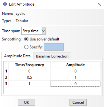
Figure 12: Cyclic amplitude
As mentioned, hysteresis strain energy and failure rate are used as criteria for crack initiation and growth. Since these parameters cannot be determined in Abaqus normally, these values must be added as keywords to the Python code of the model. These two parameters are damage initiation and damage evolution, respectively.
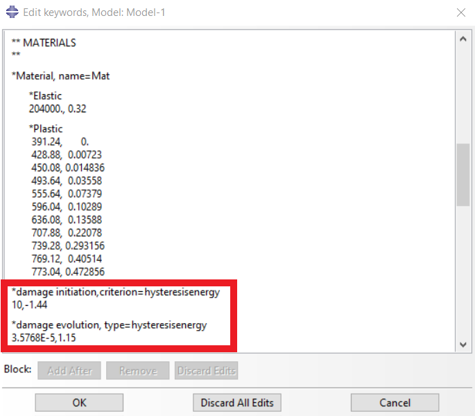
Figure 13: Damage initiation and damage evolution keywords
The numbers entered in figure 13 (10, -1.4, 3.5768E-5, and 1.15) are the constants to , respectively, for the material to determine the value of the hysteresis strain energy.
In the figure below, you can see the results of fatigue simulation using this method, where the force-time diagram appears to be cyclic.
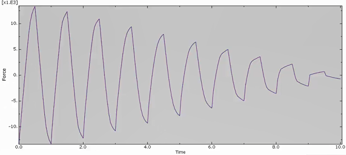
Figure 14: Force-time curve for fatigue simulation
5.2. Linear Elastic Fracture Mechanics (LEFM) Method
The second method is based on linear elastic fracture mechanics and its combination with the XFEM method, which is used to investigate the fatigue behavior of brittle materials or materials whose yield surface changes are small. In this method, there is no need to define the initial crack location, and the formation and growth of the crack and its location are predicted based on various fracture theories.
The relationship between the fracture of part (f) and the fracture energy release rate (G) at the crack tip is as follows, in which and are material constants that must be defined. If the value of (f) is greater than 1, a crack is formed in the part.
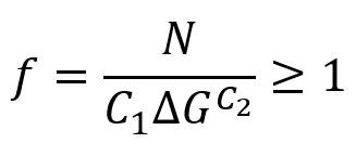
The prediction of the number of crack growth cycles in this method is done by the fracture energy release rate at the crack tip based on the Paris law and the virtual crack closure technique (VCCT). The relationship between the crack growth rate and the number of cycles with the fracture energy release rate is defined as follows, where ![]() and
and ![]() are material constants that need to be defined.
are material constants that need to be defined.
The Paris law is defined as a graph (figure 15), where G is the value of the fracture energy release rate. If the fracture energy release rate is less than Gthresh, the cracks have not yet formed. Between Gthresh and Gpl, the crack grows, and its length increases. Between Gpl and Gc the crack growth rate is accelerated and its growth rate becomes intense. After Gc, the part also fails. The ratio of Gthresh to Gc and the ratio of Gpl to Gc must be given to the software, which is considered 0.01 and 0.85 respectively by default.
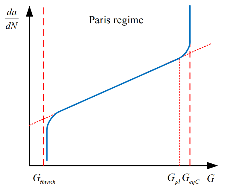
Figure 15: Paris regime [Ref]
As with the previous method, the “Direct Cyclic” step must be used in this method and fatigue adjustments must be applied to it. Also, like the previous method, in order to be cyclic, loading must be defined with an appropriate amplitude that, for example, reaches a maximum halfway through the analysis and returns to zero at the end of the cycle time.
The main difference in this method is the use of the crack generation method. To create a crack and use the XFEM method, you must enable this feature in the interaction module.
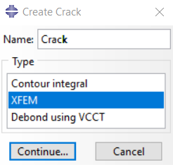
Figure 16: XFEM crack
Also, in the contact properties section, as a stress criterion, we must enable the VCCT option. This contact property is attributed to the XFEM crack.
In general, there are two methods in Abaqus for modelling behavior after the onset of failure: the displacement method and the energy method. In the energy method, unlike the displacement method, different behavior and strengths can be defined for the model in terms of normal and shear stress in different directions. The energy method in Abaqus itself is divided into three parts: the BK method, the power method, and the Reeder method; We use the BK method.
The BK method is defined as follows:
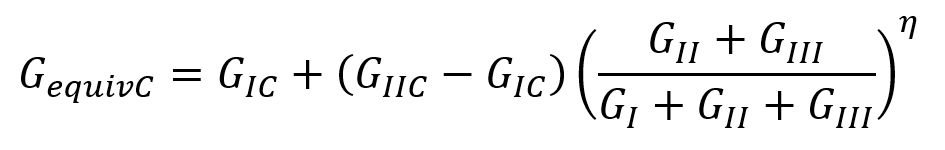
In this relation, GC means ultimate strain energy and G means fracture strain energy. Also, I, II and III indicate the normal and shear directions, respectively.
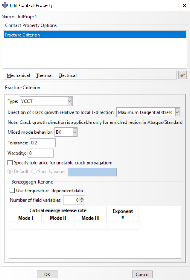
Figure 17: VCCT fracture criterion
Mode I to mode III are GI to GIII, which are equal to the normal mode fracture energy and the shear mode fracture energy in the second and third directions, respectively. The exponent n is the power value related to the BK theory, which we enter as one (Fig 17).
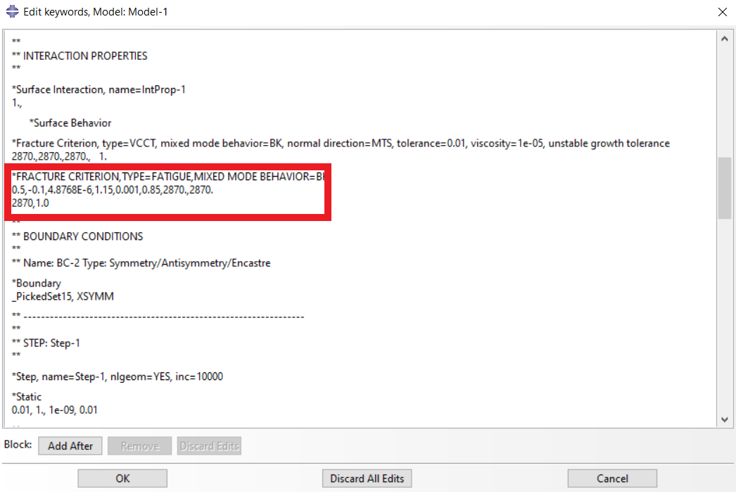
Figure 18: fracture criterion in keywords dialog
On the other hand, we must add the material constant values to the model as keywords because this is not possible graphically. See figure 18, the values 0.5, -0.1, 4.8768E-6, and 1.15 are the values of C1 to C4 respectively. Also, the values 0.001 and 0.85 are the ratio of Gthresh to Gc and the ratio of Gpl to Gc according to the Paris law respectively. On the other hand, the value 2780 has been entered for the fracture energy in three directions according to the BK model, and the power value of the BK model has been considered one.
5.3. Abaqus Fatigue with Subroutines (UMAT, VUMAT, USDFLD)
UMAT (User MATerial) is a user-defined material subroutine in Abaqus, allowing users to define custom material behavior that Abaqus does not support out of the box.
UMAT functions by computing stresses and state variables at each integration point during the analysis, based on the input strains, material properties, and internal variables. In fatigue damage simulation, UMAT can model complex fatigue behaviors such as non-linear damage, progressive crack growth, and interactions between different damage mechanisms.
The UMAT subroutine calculates the stiffness matrix to simulate fatigue in parts. First, it calculates the stiffness matrix of the material once, according to the amount of strain applied to the part and the stress. Then, according to the damage created and the failure criterion, it reduces the properties, that is, it means a reduced stiffness matrix, and step by step, the stiffness of the material decreases according to crack growth and fatigue progression. This feature of the UMAT subroutine makes the fatigue simulation not dependent on the material. This means this method is applicable to various materials such as composites and steels. In general, the use of this method has many complexities, but it is efficient and accurate.
6. Conclusion
In this article, we explored the concept of fatigue damage, focusing on how materials fail under cyclic loading. Fatigue is important to understand because it affects the lifespan and reliability of materials, which is critical in industries like aerospace, automotive, and civil engineering. Proper fatigue analysis prediction can prevent unexpected failures, ensuring the safety and longevity of components in these fields.
In this article we started by defining fatigue and discussing real-life cases such as shoe wear, bridge collapses, and machine failures. Then, we covered types of cyclic loading, including fully reversed and asymmetric, which are essential for predicting fatigue behavior. The crack growth process, the use of Paris Law for crack propagation, and fatigue life prediction through S-N curves were explained to provide a clearer understanding of how engineers estimate material life. Also, we have learned where to start Abaqus Fatigue analysis.
Overall, this article highlighted the importance of recognizing fatigue damage early, the mechanisms behind it, and how different loading conditions impact material failure. Understanding these principles helps in designing more resilient components and improving safety in various industries.
Now, it is time to practice what we have learned here; we have 2 essential examples: 2D & 3D Fatigue crack growth simulation along with all simulation files. You can see the details in each example below.
|
|
Explore our comprehensive Abaqus tutorial page, featuring free PDF guides and detailed videos for all skill levels. Discover both free and premium packages, along with essential information to master Abaqus efficiently. Start your journey with our Abaqus tutorial now!
The CAE Assistant is committed to addressing all your CAE needs, and your feedback greatly assists us in achieving this goal. If you have any questions or encounter complications, please feel free to share it with us through our social media accounts including WhatsApp.
You can always learn more about Abaqus fatigue analysis from Abaqus Documentation.