
Abaqus Welding Simulation Complete Guide: Essential Methods and Theories Explained

Abaqus welding simulation is crucial when predicting the impact of welding on materials. It helps engineers understand heat effects, deformation, material distortion, and residual stresses. This is particularly useful in complex welding situations, where traditional methods may not provide accurate results. Abaqus allows for a detailed analysis of thermal distribution and material behavior, making it an essential tool in the welding process.
Abaqus uses several techniques to model welding, such as heat flux configurations and the DFLUX subroutine for custom thermal conditions. The “death and birth of elements” method is also key, enabling material addition as the weld progresses. The software uses various theoretical approaches like Lagrangian, Eulerian, and ALE methods to accurately simulate material flow and deformation during welding, ensuring realistic results.
This blog covers Abaqus welding simulations step by step. You’ll explore how to use different simulation methods and apply them in practice, like creating parts and setting material properties. It also explains the theoretical methods used to track material deformation. Finally, the blog introduces welding methods, from fusion to non-fusion techniques, showing their real-world applications in industries like aerospace and automotive.
Want to practice welding simulations in Abaqus? You’re in the right place! These tutorials cover over 10 types of welding simulations, from basic to advanced, each designed to replicate real-world welding techniques like arc welding, friction stir welding, and inertia welding. But that’s not all! You’ll learn the types of welding and the methods and theories behind the scenes of the simulations.
|
Welding types + Theories and Elements in Abaqus Welding Simulation + Welding Simulation Methods in Abaqus + 6 different workshops (butt welding, explosive welding, etc.) |
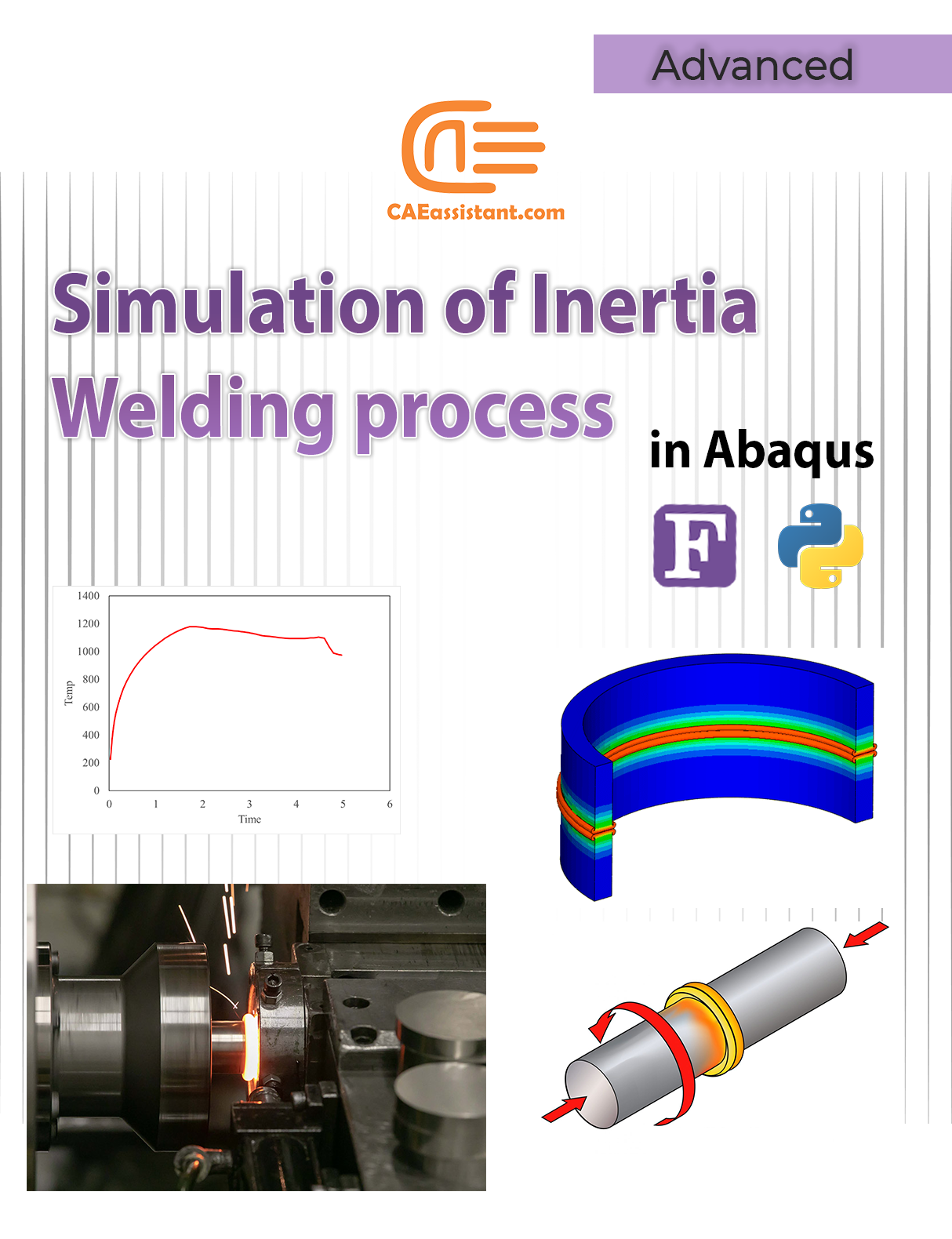
simulate rotary friction welding, heat is generated through rotational motion and pressure. Heat generation, material deformation, and phase transformation. |
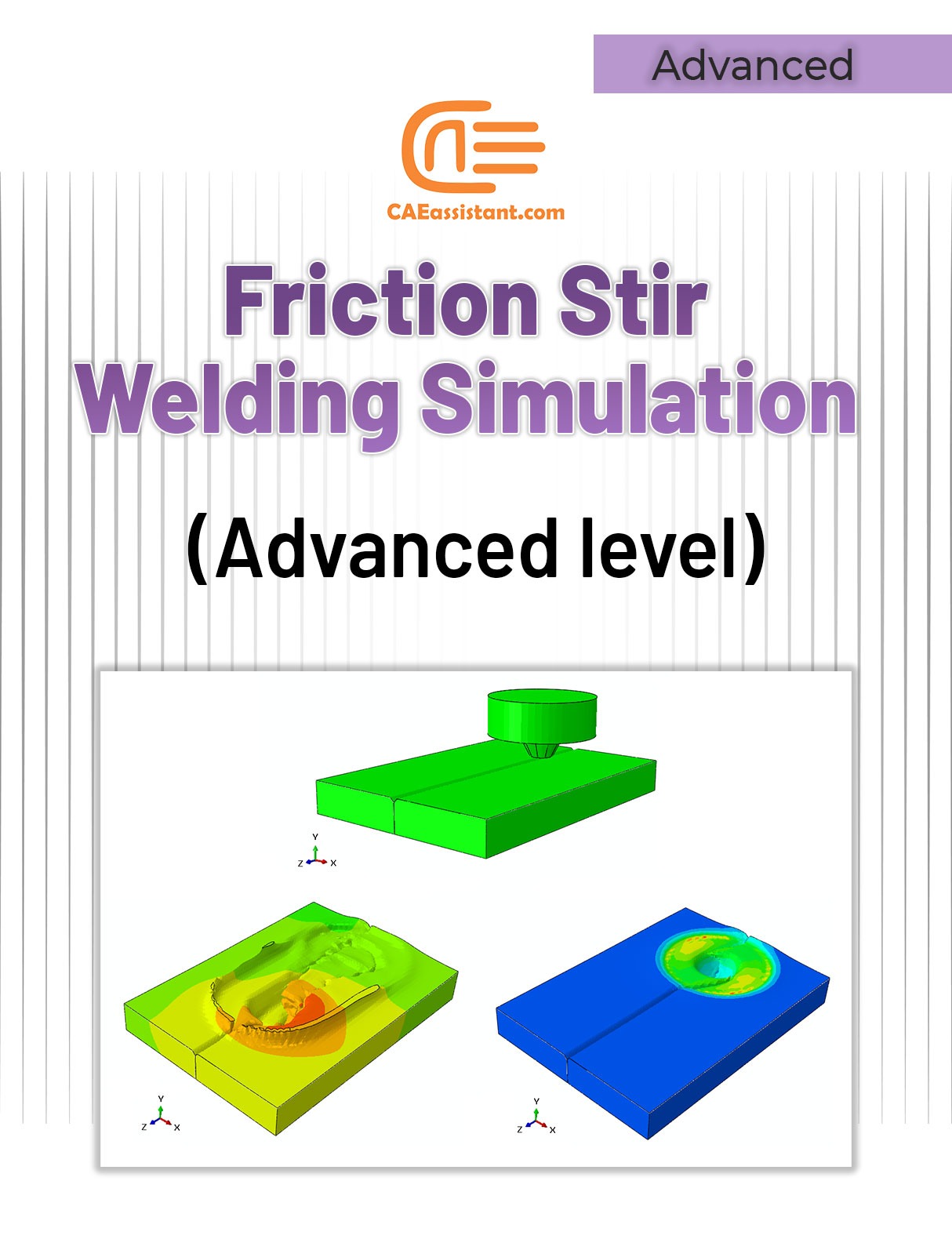
Friction Stir Welding (FSW) – Advanced Level – Take your FSW simulation skills to the next level with advanced techniques and insights. |
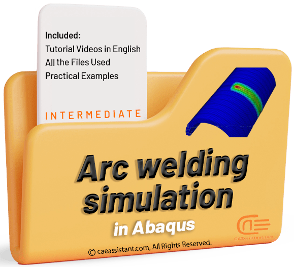
Moving heat source method to simulate arc welding in Abaqus. model heat transfer, molten pool dynamics, and residual stresses. 3 Examples |
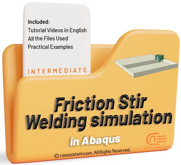
Friction Stir Welding (FSW) – Basic Level – Get started with FSW simulation with 6 Examples, understanding material flow and joint formation |
1. Abaqus Welding Simulation Methods
There are several Abaqus welding simulation approaches, such as heat flux configuration, custom subroutines, progressive material addition, and advanced thermal modeling for accurate and realistic process representation. These methods form the basis for simulating welding in Abaqus.
- Direct Settings
Direct setting configures heat flux, material properties, and boundary conditions directly within Abaqus for straightforward simulations.
Allows user-defined heat flux distributions to simulate complex thermal conditions during welding in Abaqus.
- Death and Birth of Elements
Simulates material addition or removal by activating or deactivating mesh elements progressively.
- Surface and Volumetric Thermal Flux
Applies heat flux to specific surfaces or volumes, allowing precise thermal modeling in Abaqus welding simulations.
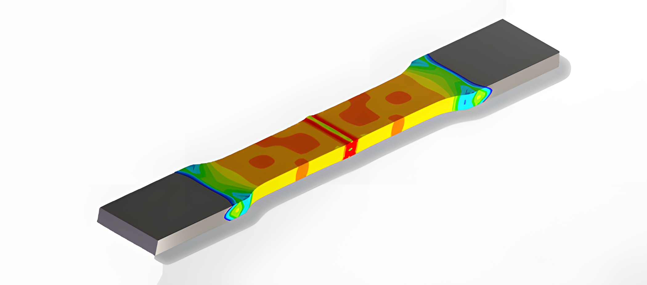
Figure 1: Abaqus Welding simulation
All of these simulation methods and more are covered in the lesson of our tutorial package “What are welding simulation methods?“.
1.1. Welding Simulation with DFLUX Subroutine
In Abaqus, the DFLUX subroutine allows users to define custom heat flux distributions within their welding simulation.
This capability is essential for accurately modeling complex thermal conditions in welding processes, enabling the simulation of localized heating effects and transient thermal behaviors that standard predefined options may not capture.
1.2. What is the Method of Death and Birth of Elements?
The “death and birth” method in Abaqus refers to the technique of deactivating (killing) and reactivating (birthing) elements during a simulation.
This approach is particularly useful in Abaqus welding simulations to represent the addition of new material as the weld progresses, allowing for a more realistic depiction of the welding process and its effects on the overall structure.
All of the mentioned methods on the left side are fully explained in simple terms in the Abaqus full welding tutorial along with examples and simulation files.
1.3. What is the Surface Volumetric Thermal Flux Method?
The surface volumetric thermal flux method in Abaqus involves applying heat flux either on the surface or throughout the volume of the model.
This is crucial for accurately simulating the thermal aspects of welding processes, as it allows for the representation of heat input distribution, which directly affects the thermal gradients and subsequent material behavior during and after welding.
1.4. Resistance Welding in Abaqus
Resistance welding, a widely used method, combines heat from electric current and mechanical pressure. Simulating this process in Abaqus can be challenging due to complexities in modeling electric-thermal interactions and pressure application.
Figure 2: Resistance welding [Ref]
2. Example of Welding in Abaqus: Step by Step guide
We are going to show you an example of welding in Abaqus as to how the simulation is done to determine the answer for your project.
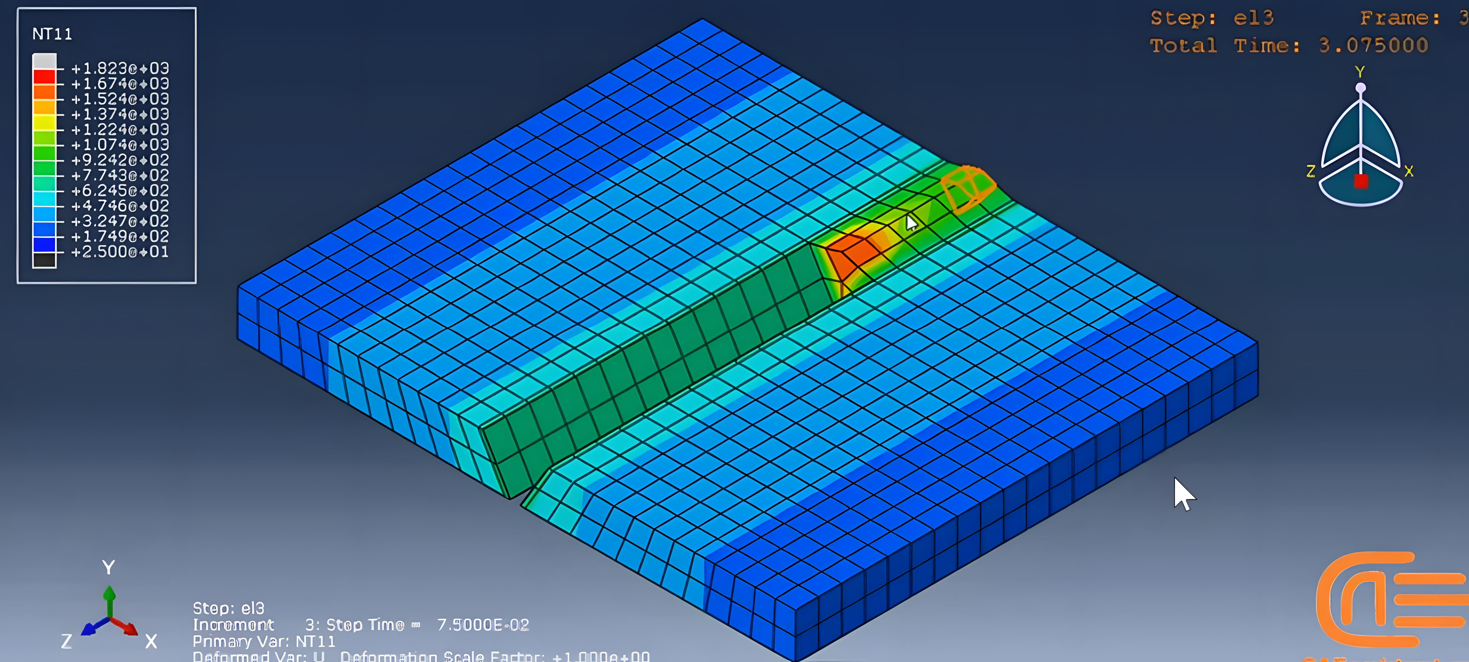
Figure 3: Abaqus Butt welding with death and birth of an element
Butt welding with death and birth of an element method is a challenging simulation in Abaqus but do not worry we will show how the simulation works in our workshop. There are certain elements specified for this simulation which we will use to run our simulation.
2.1. Creating Parts and Dimensions
The weld part based on the dimensions on figure 4 created, and the two base metal part will be placed together to form an assembly. The wield part will be added gradually in the welding process, which are several small parts.
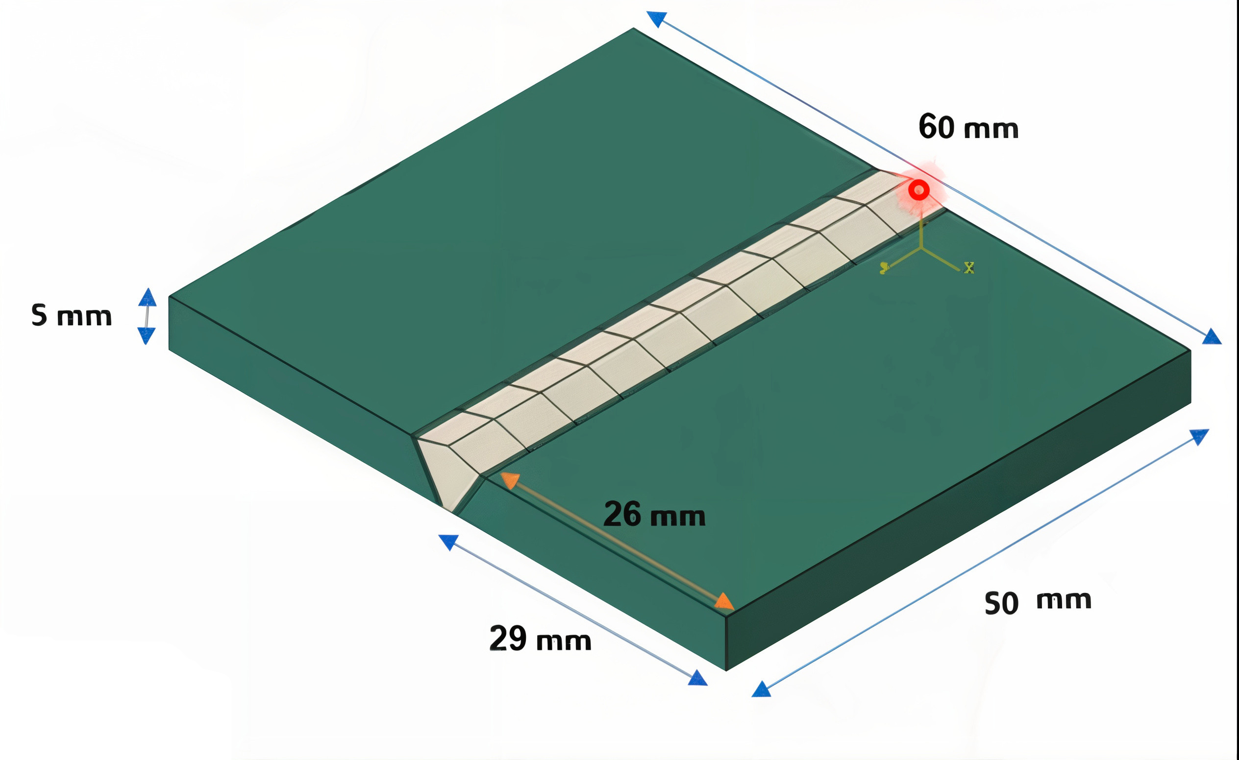
Figure 4: The base of the metal parts and the weld
The based sketched as 3D solid with the deformable, and solid (extrusion). Then the weld part will be created and assembled.
2.2. Material Properties
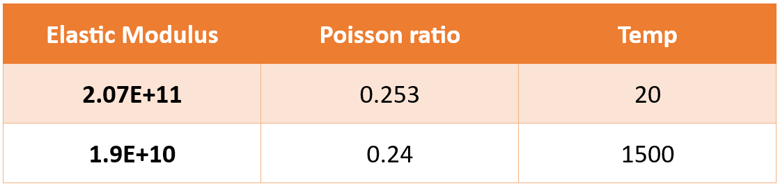
The expansion coefficient at temperature 100 degree is 1.19e-5 and at the 5000 degree is 1.38e-5 which we use on our simulation.
The elastic modulus unit is pascal and presented in this table:
We need to define latent heat, solidus temperature, and liquidus temperature because there is melting. The solidus is the highest temperature at which an alloy is completely solid. The liquidus is the lowest temperature at which an alloy is completely liquid. The latent heat is the energy released during the welding process.

First the two plates are put together, then the weld part will be added gradually when the process is started.
2.3. Step Definition
Define of the death and birth of an element is defined here in the step module. Now we need to define 12 steps for this analysis due to using birth and death of element method. In the inactive step there are only the base metal and the weld, which its work is to allow the static status phase of the base metal and then the weld. After that, in the 10 next step the welding will be in progress. Lastly the cooling step is defined for the cooling purpose which will be explained later on.
Why ten steps?
As you see in the figure 4 the weld elements are 10 parts, this is why we choose 10 of these steps as they are ten elements set to be created in the process, shown in figure 5.
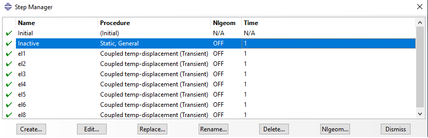
Figure 5: The steps created for 10 elements
In each of the steps given for the birth the steps will be transient and liner. Also, by setting the temperature in this case to 2000 centigrade.
Note that all steps except for the first one must be coupled. Also, the solver must be standard. Because we use model change interaction for the birth of an element method.
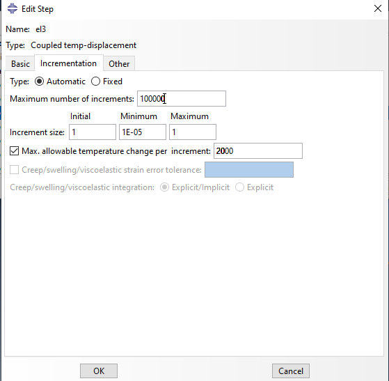
Figure 6: step setting
The first step is the Static General type nonlinear geometry is off, and other settings are by defaults. Th next ten steps named “el1” to “el10”, and their settings are the same just like figure 6. The nonlinear geometry is off. Select transient response because the temperature will change during the process. Set the maximum allowable temperature change per increment to 2000. Other settings are by default.
Finally, the last step which called the cooling phase (step) will be the cooling phase to be applied with 100 seconds so the process will be completed. In the field output request editor, we use the default output variables.
Now you can see why we needed 12 steps.
2.4. Interaction
We must define the condition of each part in contact to the other during the simulation in this module. In each step we select one weld element at a time and doing the rest for all the defined steps.
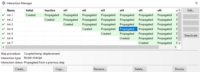
Figure 7: interactions
Open the interaction manager dialogue box, in the first step named inactive, all weld elements are inactive. Select the Geometry from the region type, and select all weld parts. Then select the deactivated in this step.
In the next 10 steps, we activate one weld element at a time. For each, create new interaction, select the model change. Choose the inactive step, name the interaction, and click continue. The settings are the same as we have explained, and now select the weld parts, and click done.
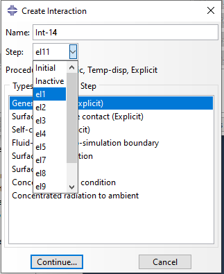
Figure 8: active and inactive
Now we must activate one weld element in the next step. Select the Model change again, select the first weld element, and select reactivate in this step. Do this for the other 9 remaining weld elements. Now, just delete the extra interactions and go to the next module.
2.5. Loading and Boundary Conditions
We fix the right side of the model by using the Encastre. This boundary condition is active from the beginning of the analysis till the end. Next, we create the load for the all 10 steps which the Abaqus welding is under progress. The type of the load is the “Body heat flux” with the magnitude of 5e9 with a uniform distribution. This head flux is applied instantaneously.
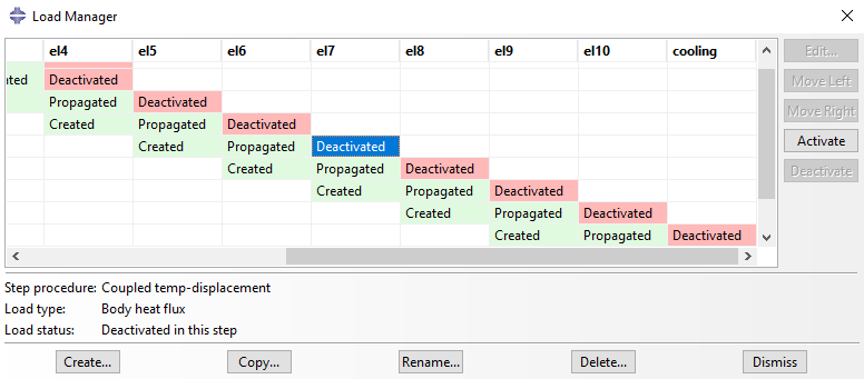
Figure 9: Load manager based on the steps for each element
The other 9 steps have this loading condition as well shown in figure 9. Note that each body heat flux is active only till the next step and will be inactive afterwards. As the welding pen moves forward and the heat generated from the welding pen concentrates only in the pen surrounding. Also, the body heat flux will be inactive in the cooling step.
Also do note that you need to deactivate previous the body heat flux load for so in order to mimic the welding simulation shown in figure 9.
Let’s create one load to show you how it’s done. In the create load dialog box, select Thermal from the category, select body heat flux, and click continue. Select the first weld element, enter the 5e9 in the magnitude field, and click OK. We keep this load active only to the next step. Do the same for the next steps. Again, the load remains active only to the next step.
Next, we must define the initial temperature. The initial temperature of the parts between the weld and the base metal is 25 degrees. But the initial temperature of the weld element is 1500 degrees centigrade because it is the liquidus temperature.
There are more examples in our Abaqus full welding tutorial along with examples and simulation files; such as Explosive Welding
2.6. Meshing
Now let’s mesh the model. We mesh the parts in figure 10 one by one. We use the structural technique to mesh the model. The approximate global size is 0.0025, hexagonal and structured based. And the element type is standard coupled temperature displacement with liner geometry (C3D8T).
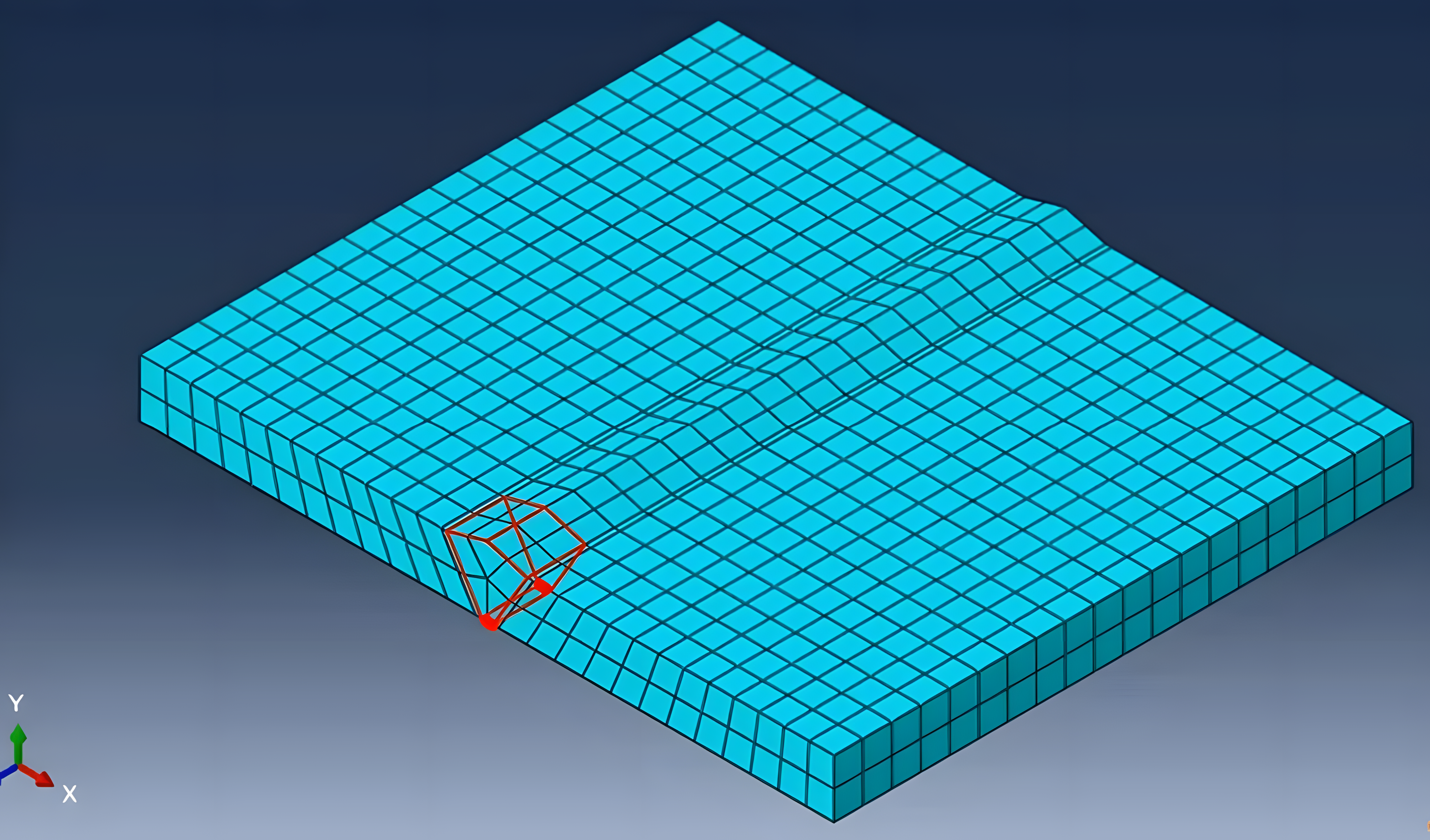
Figure 10: Meshing the parts
Then the element type will be defined as coupled temperature displacement as the element family type.
2.7. Job and Results
Next, we run the job simulation to determine the results. Then on the visualization module we select what we need to see, which is the exterior edges and their deformation or we can select the animation to see the video of the welding simulation video. If you needed to adjust it, you may use animation option to alter any customization.
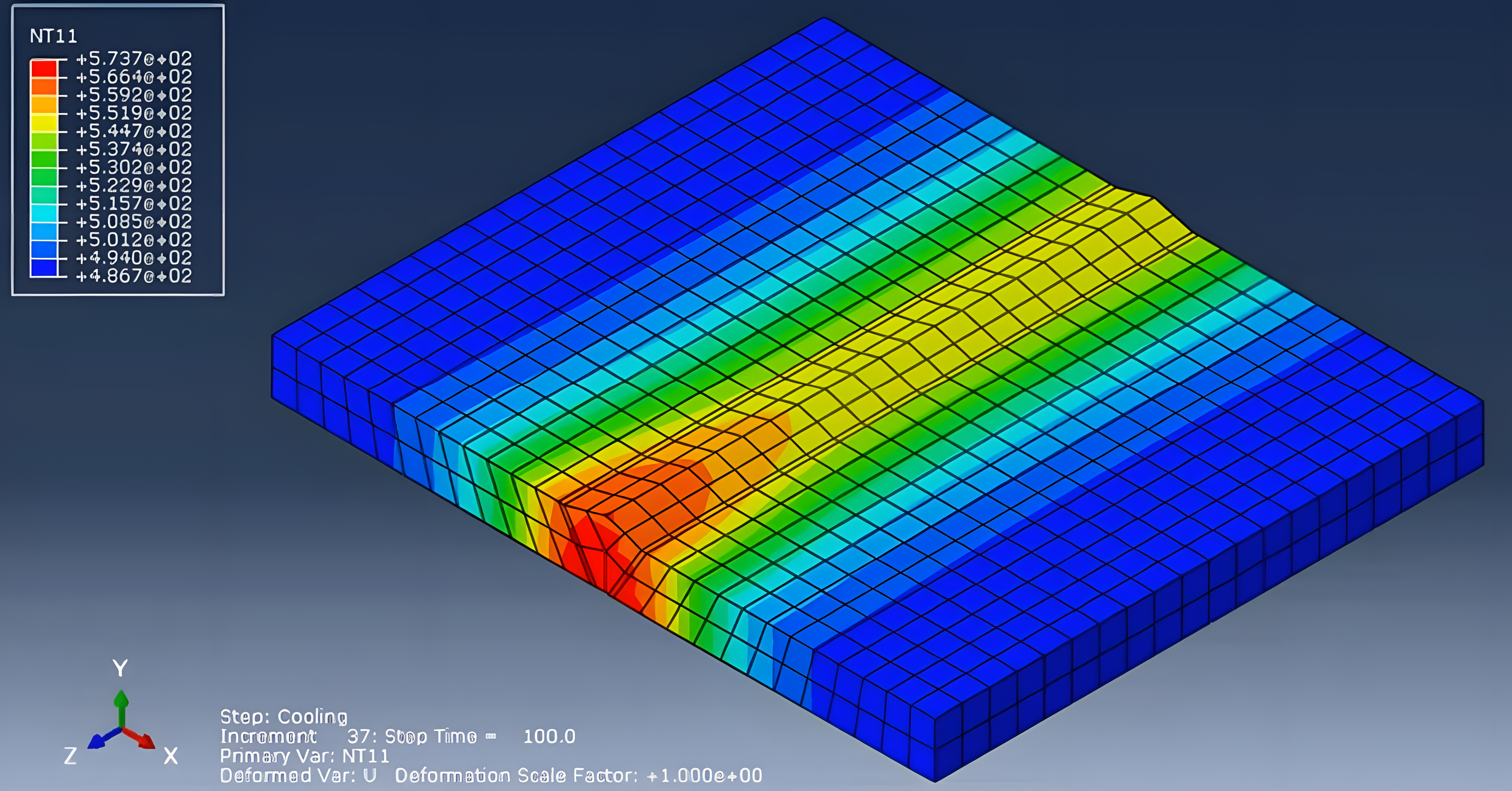
Figure 11: Simulation results
By playing the weld element will appear gradually forming the actual welding simulation. Considering that our analysis is transient, some contours like stress and temperature will change during solution steps. You can select the nodal temperature from the field output variables to see the temperature distribution in the contour plots. In figure 11 you see, the initial temperature is 1500 degree centigrade. The temperature will be applied only to the current weld element when welding is in progress because the analysis is transient.
If you want to gain access to the full information on how to setup this Abaqus welding simulation see the workshop “Butt welding with death and birth of an element method“.
3. Element and Theories in Welding Simulation
This section explores four key theoretical methods—Lagrangian, Eulerian, ALE, and SPH—used in Abaqus welding simulations to handle different deformation and material flow scenarios effectively.
Welding simulations in Abaqus utilize four main theoretical approaches which allows to determine the thermal effect like thermal distribution, heat affected zones, cooling rates.
In welding problem, we typically want to know if the structure is resilient enough to the temperatures created. The temperature or thermal distribution during the welding process will be determined using theories of heat transfer equation. (Figure 12)
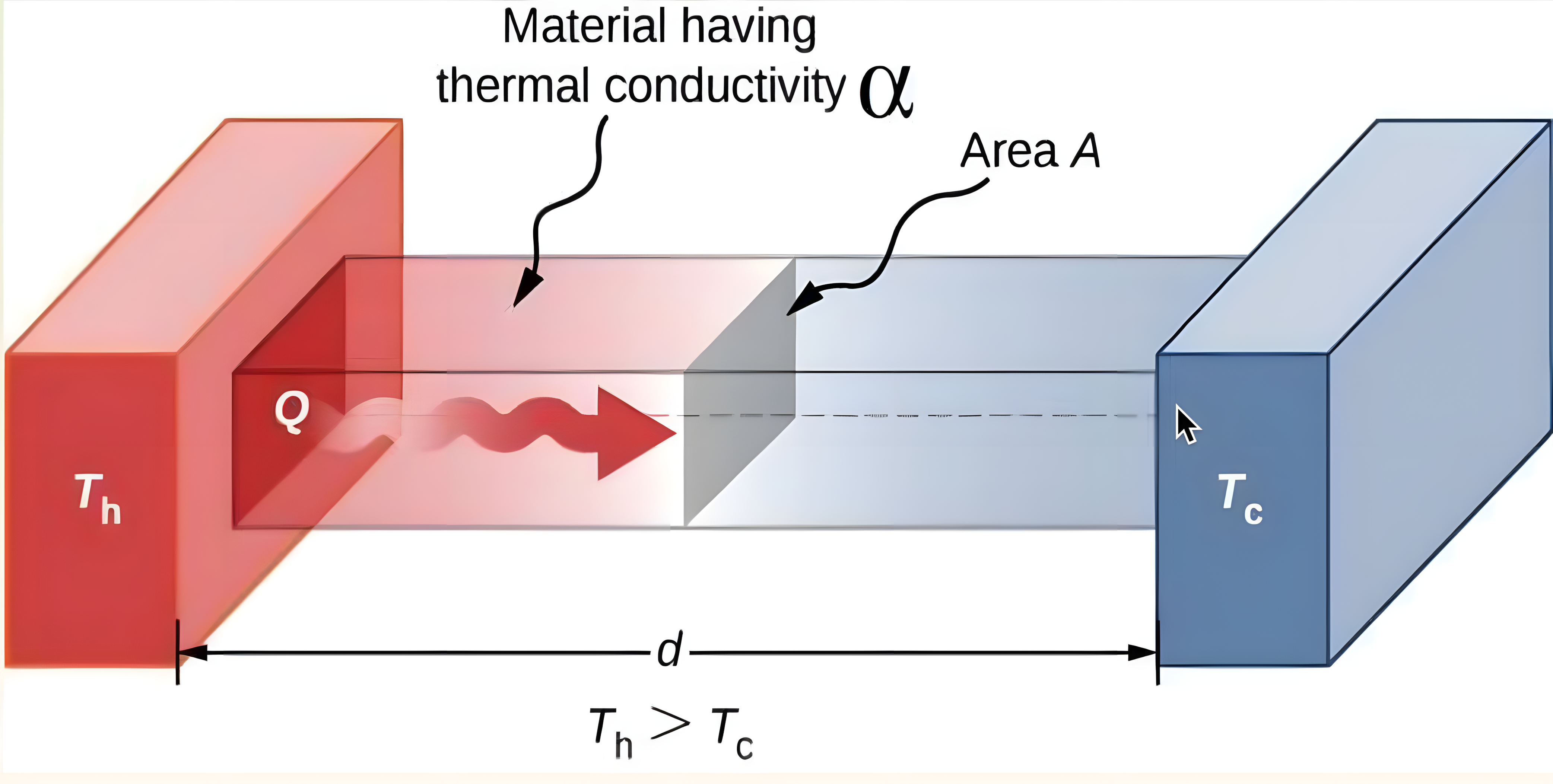
Figure 12: Heat transfer during welding [Ref]
However, for deformation determination or simply the strain of materials during welding the classical theories use which we mention their names below.
- Lagrangian theory
- Eulerian theory
- Arbitrary Lagrangian-Eulerian (ALE)
- Smoothed Particle Hydrodynamics (SPH)
3.1. What is the Lagrangian Theory?
The Lagrangian method in welding simulation tracks material deformation by attaching the computational mesh to the material itself, and is ideal for solid mechanics problems, as it simplifies the application of boundary conditions.
However, under high deformation, the mesh can become distorted, leading to inaccuracies in the simulation results. Therefore, careful mesh management is essential when using this method.
3.2. What is the Eulerian Theory?
In the Eulerian method, the computational mesh remains fixed in space while the material flows through it. This approach is particularly good in scenarios involving large deformations, as it prevents mesh distortion.
However, accurately tracking interfaces and free surfaces can be challenging, requiring sophisticated algorithms to ensure precise material representation. (see figure 13)
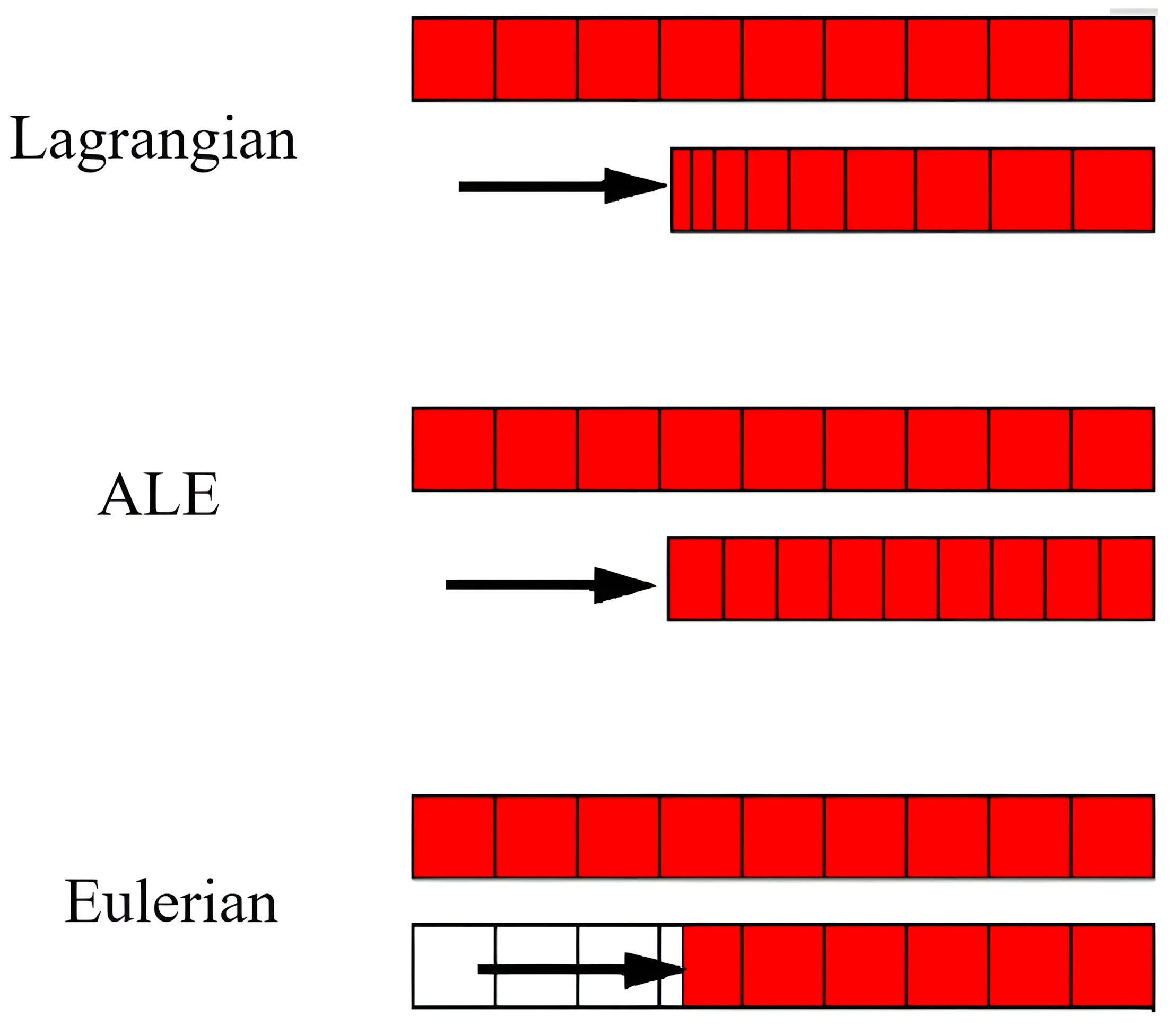
Figure 13: Motion of mesh and material with various methods
3.3. What is the ALE Theory?
The Arbitrary Lagrangian-Eulerian method combines aspects of both Lagrangian and Eulerian approaches. In this method, the mesh can move independently of the material, allowing for flexibility in handling large deformations while minimizing mesh distortion.
This versatility makes ALE particularly useful in welding simulations where both material flow and structural integrity are critical.
3.4. What is the SPH Theory?
Smoothed Particle Hydrodynamics is a mesh-free method that represents the material as a collection of particles.
Each particle carries properties such as mass, velocity, and temperature. SPH is especially suited for simulating phenomena involving extreme deformations, high strain rates, or complex free surface flows, such as explosions or fluid splashing, where traditional mesh-based methods may fail.
4. What Are the Welding Methods?
Welding methods can be broadly categorized into two primary types, Fusion welding (melting) and Non-Fusion welding (non-melting) . Both methods are essential in modern welding simulations in the industry.
Each method has unique mechanisms, applications, and considerations. So, let’s review them together! Just remember, most of the welding methods in industry are explained with their advantages and disadvantages and their specific features are covered in the Full welding tutorial.
4.1. How is the Fusion welding performed?
Fusion welding or melting method involves using heat to melt and join materials, allowing them to bond upon cooling. This process may or may not require filler materials which is the material used to fill the gap between the two components and act as a connector in welding. We will give an example for each so keep reading down below!
Here are some common examples in Fusion category:
- Electron Beam Welding (EBW)
Electron Beam Welding (EBW) uses high-energy electrons to melt and join materials, offering exceptional precision and penetration. It operates in a vacuum, reducing contamination and enabling deep welds. Unlike arc or laser welding, EBW is ideal for thick sections, making it highly suited for aerospace and automotive industries requiring precise, defect-free joints.
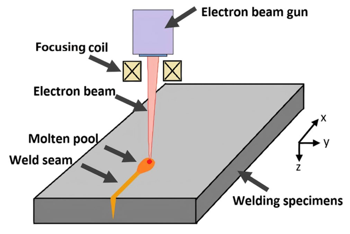
Figure 14: EBW [Ref]
Electron Beam Welding (EBW) is widely applied in aerospace, automotive, nuclear, electronics, and medical industries for precision joining and defect-free welds in critical components.
- Laser Beam Welding (LBW)
Laser Beam Welding (LBW) employs laser beams for precise, deep, and narrow welds without filler materials, ideal for delicate applications. It uses focused laser energy to join metals, offering higher precision than arc welding. LBW excels in automated, high-speed operations, especially for thin materials, making it suitable for aerospace and electronics industries.
LBW is widely used in aerospace, automotive, electronics, and medical industries for high-precision, automated, and defect-free welding of thin materials and intricate components.
- Arc Welding
Arc welding in Fig. 15 generates heat through an electric arc, making it versatile and widely used in industries. It uses an electric arc between an electrode and base metal to create intense heat. Unlike laser or electron beam welding, it’s less precise but cost-effective and adaptable. Arc welding has several subtypes, including TIG, MIG, and submerged arc welding.
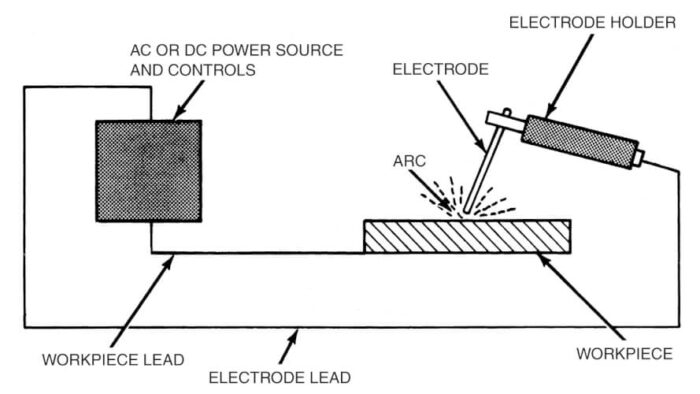
Figure 15: arc welding [Ref]
Arc welding is extensively applied in construction, automotive, shipbuilding, pipeline, and general manufacturing industries for its versatility and cost-effective joining of metals.
4.2. How is the non-fusion welding done?
In contrast non-melting welding method uses pressure or a combination of heat and pressure without melting the base martials.
Non-fusion welding or non-melting method relies on pressure and, occasionally, heat to join materials without melting them.
Examples of Non-fusion welding include:
- Friction Stir Welding (FSW)
It uses a rotating tool to generate frictional heat and mechanical pressure, softening the materials without melting them. This solid-state process ensures high-strength, defect-free joints with minimal distortion, making it ideal for critical applications such as aircraft panels, car body structures, and railway carriages. shown in Fig. 16.
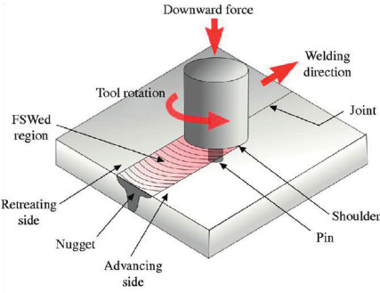
Figure 16: FSW [Ref]
FSW is widely used in aerospace, automotive, shipbuilding, railways, and electronics industries for joining lightweight materials like aluminum and magnesium.
- Explosive Welding
The explosive welding method utilizes controlled explosive energy to join materials through high-velocity impact.
In Abaqus, simulating this process involves modeling the rapid pressure application and the resulting material deformation, requiring precise definition of material properties and interaction behaviors to accurately capture the welding dynamics.
- Ultrasonic Welding
In figure 17 ultrasonic welding uses high-frequency vibrations to create solid-state welds without melting materials, making it ideal for plastics and thin metals. The process generates heat through friction at the interface, forming strong bonds. Unlike fusion methods, it avoids thermal damage to surrounding structures, offering precision and reliability, particularly in electronics, medical devices, and packaging industries.
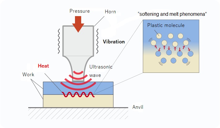
Figure 17: Ultrasonic Welding [Ref]
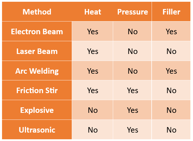
The table below summarizes the heat and pressure requirements for various welding methods:
Want to practice welding simulations in Abaqus? You’re in the right place! These tutorials cover over 10 types of welding simulations, from basic to advanced, each designed to replicate real-world welding techniques like arc welding, friction stir welding, and inertia welding. But that’s not all! You’ll learn the types of welding and the methods and theories behind the scenes of the simulations.
|
Welding types + Theories and Elements in Abaqus Welding Simulation + Welding Simulation Methods in Abaqus + 6 different workshops (butt welding, explosive welding, etc.) |
simulate rotary friction welding, heat is generated through rotational motion and pressure. Heat generation, material deformation, and phase transformation. |
Friction Stir Welding (FSW) – Advanced Level – Take your FSW simulation skills to the next level with advanced techniques and insights. |
Moving heat source method to simulate arc welding in Abaqus. model heat transfer, molten pool dynamics, and residual stresses. 3 Examples |
Friction Stir Welding (FSW) – Basic Level – Get started with FSW simulation with 6 Examples, understanding material flow and joint formation |