Cohesive Elements in Abaqus: An Introduction

Cohesive elements are specialized finite element types used in Abaqus to model the behavior of interfaces between two or more materials. They are particularly useful for capturing the failure and debonding of adhesive bonds, composites, and other layered structures.

Abaqus offers a library of cohesive elements to model the behavior of adhesive joints, interfaces in composites, and other situations where the integrity and strength of interfaces may be of interest.

In this article, we are going to have an overall review of different aspects of cohesive elements to have better insight for modeling them in your Abaqus analyses.

1. Abaqus Cohesive Elements Modeling

Modeling with cohesive elements in Abaqus consists of:

• Choosing the appropriate cohesive element type
• Including the cohesive elements in a finite element model, connecting them to other components, and understanding typical modeling issues that arise during modeling using cohesive elements
• Defining the initial geometry of the cohesive elements
• Defining the mechanical, and optionally the fluid, constitutive behavior of the cohesive elements.

1.1. Cohesive elements application

Cohesive elements are useful in modeling adhesives, bonded interfaces, gaskets, and rock fractures. The constitutive response of these elements depends on the specific application and is based on certain assumptions about the deformation and stress states that are appropriate for each application area.

The nature of the mechanical constitutive response may broadly be classified to be based on one of the following:

• Continuum description of the material
• Traction-separation description of the interface
• Uniaxial stress state appropriate for modeling gaskets and/or laterally unconstrained adhesive patches.

Each of these constitutive response types will be discussed briefly.

1.2. Abaqus Cohesive Zone Models

Cohesive zone modeling predicts the behavior within the cohesive element (or cohesive contact) and the adhesion between the cohesive element and parent elements is perfect. When we talk about the cohesive zone model (CZM), maybe you first consider the traction-separation model which is commonly used in modeling crack fracture, but as we mentioned, the mechanical constitutive response of the cohesive zone or cohesive zone models can be classified into three different groups.

1.2.1. Continuum-based modeling

The modeling of adhesive joints involves situations where two bodies are connected together by a glue-like material as shown in figure 1. A continuum-based modeling of the adhesive is appropriate when the glue has a finite thickness.

The macroscopic properties, such as stiffness and strength, of the adhesive material can be measured experimentally and used directly for modeling purposes. The adhesive material is generally more compliant than the surrounding material.

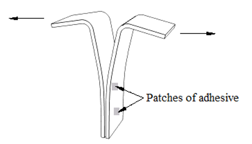
Figure 1: Typical peel test using cohesive elements to model finite-thickness adhesives

In three-dimensional problems, the continuum-based constitutive model assumes one direct (through-thickness) strain, two transverse shear strains, and all (six) stress components to be active at a material point.

In two-dimensional problems, it assumes one direct (through-thickness) strain, one transverse shear strain, and all (four) stress components to be active at a material point.

1.2.2. Traction-separation-based modeling

The modeling of bonded interfaces in composite materials often involves situations where the intermediate glue material is very thin and for all practical purposes may be considered to be of zero thickness (Figure 2).

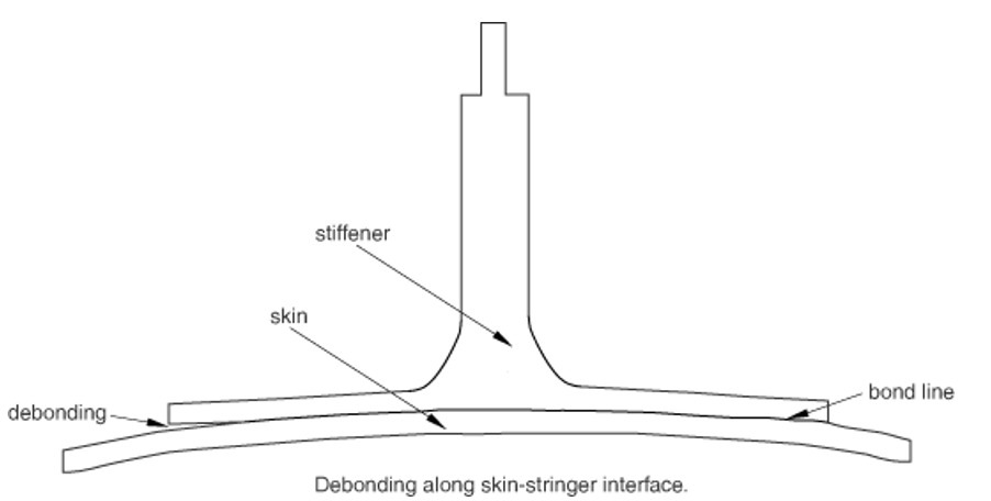
Figure 2: Debonding along a skin-stringer interface: typical situation for traction-separation-based modeling

In three-dimensional problems, the traction-separation-based model assumes three components of separation—one normal to the interface and two parallel to it; and the corresponding stress components are assumed to be active at a material point.

In two-dimensional problems the traction-separation-based model assumes two components of separation—one normal to the interface and the other parallel to it; and the corresponding stress components are assumed to be active at a material point.

1.2.3. Modeling of gaskets and/or laterally unconstrained adhesive patches

Cohesive elements also provide some limited capabilities for modeling gaskets (Figure 3). The constitutive response of gaskets modeled with cohesive elements can be defined using only macroscopic properties such as stiffness and strength. No specialized gasket behavior (typically defined in terms of pressure versus closure) is available.

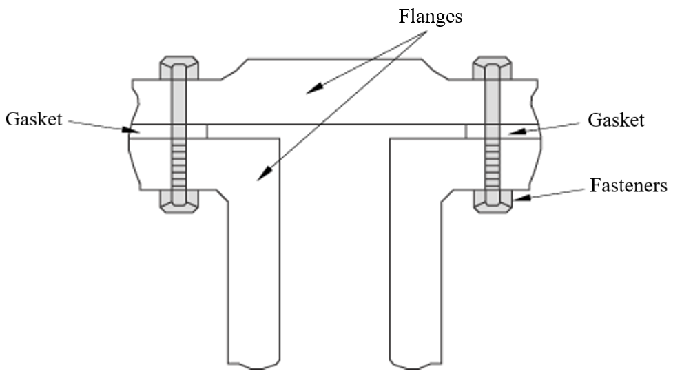
Figure 3: Typical application involving gaskets

Compared to the class of gasket elements available in Abaqus/Standard, the cohesive elements:

• are fully nonlinear (can be used with finite strains and rotations)
• can have mass in a dynamic analysis
• are available in both Abaqus/Standard and Abaqus/Explicit

It is assumed that the gaskets are subjected to a uniaxial stress state. A uniaxial stress state is also appropriate for modeling small adhesive patches that are unconstrained in the lateral direction.

1.3. Representation of a cohesive element

The key geometrical features that are used to define cohesive elements are shown in figure 4.

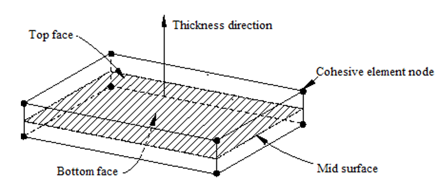
Figure 4: Spatial representation of a three-dimensional cohesive element

The connectivity of cohesive elements is like that of continuum elements, but it is useful to think of cohesive elements as being composed of two faces separated by a thickness. The relative motion of the bottom and top faces measured along the thickness direction represents the opening or closing of the interface.

The relative change in position of the bottom and top faces measured in the plane orthogonal to the thickness direction quantifies the transverse shear behavior of the cohesive element. Stretching and shearing of the mid surface of the element (the surface halfway between the bottom and top faces) are associated with membrane strains in the cohesive element; however, it is assumed that the cohesive elements do not generate any stresses in a pure membrane response.

The different deformation modes of a cohesive element are shown in figure 5.

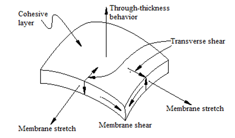
Figure 5: Deformation modes of a cohesive element

If you need practical examples or more info about cohesive and cohesive elements in Abaqus, I recommend watch this tutorial:

“Implementation of Cohesive by interaction & element based methods in ABAQUS”

2. Abaqus cohesive elements library

The Abaqus cohesive element library includes elements for two- and three-dimensional analyses, and also for axisymmetric analyses.

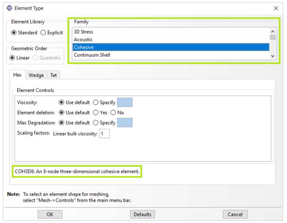
Figure 6: Selecting a cohesive element in Abaqus

The cohesive elements used in Abaqus are named as shown in figure 7.

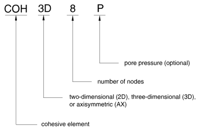
Figure 7: Abaqus cohesive elements naming convention

3. Modeling cohesive zones

The cohesive zone must be discretized with a single layer of cohesive elements through the thickness.

• If the cohesive zone represents an adhesive material with a finite thickness, the continuum macroscopic properties of this material can be used directly for modeling the constitutive response of the cohesive zone.
• If the cohesive zone represents an infinitesimally thin layer of adhesive at a bonded interface, it may be more relevant to define the response of the interface directly in terms of the traction at the interface versus the relative motion across the interface.
• If the cohesive zone represents a small adhesive patch or a gasket with no lateral constraint, a uniaxial stress state provides a good approximation of the state of these elements.

At least one of either the top or the bottom face of the cohesive element must be constrained to another component. In most applications, it is appropriate to have both faces of the cohesive elements tied to neighboring components. In some cases, it may be convenient and appropriate to have cohesive elements share nodes with the elements on the surfaces of the adjacent components.

More generally, when the mesh in the cohesive zone is not matched to the mesh of the adjacent components, cohesive elements can be tied to other components. When cohesive elements are used to model gaskets, it may be more appropriate to tie or share nodes on one side and define contact on the other side; This will prevent the gaskets from being subjected to tensile stresses.

3.1. Cohesive elements share nodes with other elements

When the cohesive elements and their neighboring parts have matched meshes, it is straightforward to connect cohesive elements to other components in a model simply by sharing nodes as shown in figure 8.

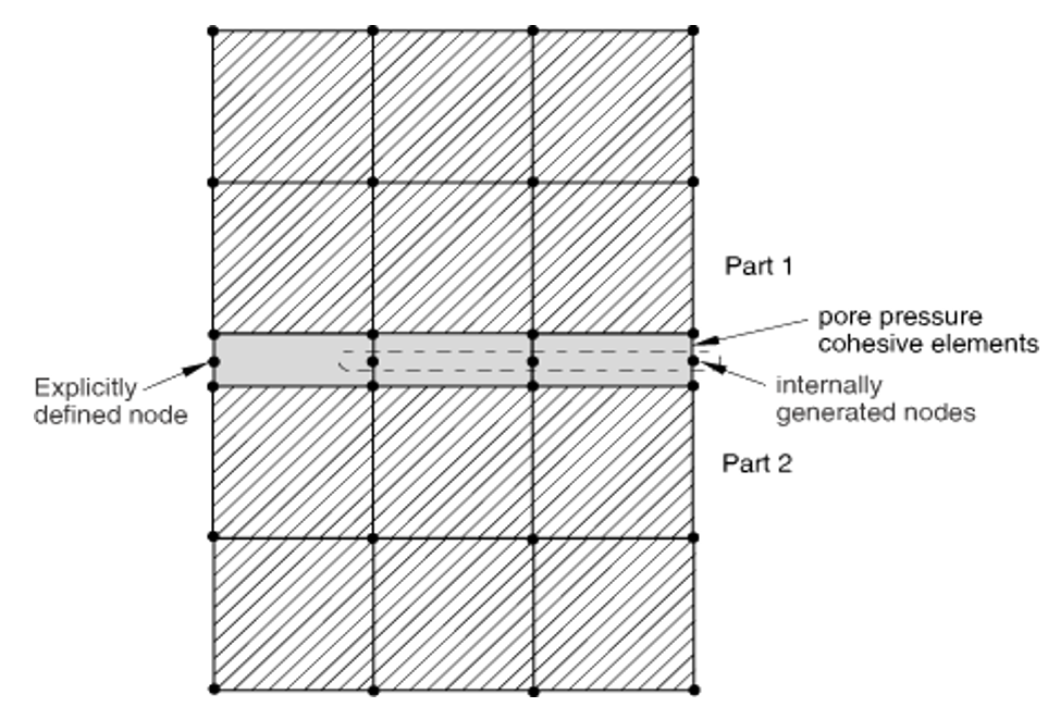
Figure 8: Cohesive elements sharing nodes with other Abaqus elements

The method of sharing nodes in gasket applications will lead to tensile stresses in the gasket should the parts connected to the gasket be pulled apart. Defining contact on one side of the cohesive elements will avoid such tensile stresses.

3.2. Cohesive elements connected to other components by using surface-based tie constraints

If the two neighboring parts do not have matched meshes, such as when the discretization level in the cohesive layer is different (typically finer) from the discretization level in the surrounding structures, the top and/or bottom surfaces of the cohesive layer can be tied to the surrounding structures using a tie constraint (Figure 9).

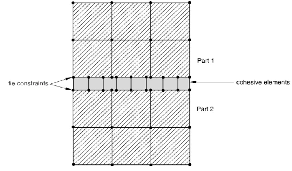
Figure 9: Independent meshes with tie constraints

3.3. Contact interactions between cohesive elements and other components

For some applications involving gaskets, it is appropriate to define contact on one side of the cohesive element (Figure 10). If pure master-slave contact is used, typically the surface of the cohesive elements should be the slave surface and the surface of the neighboring part should be the master surface. This choice of master and slave is based on the cohesive zone typically being composed of softer materials and having a finer discretization.

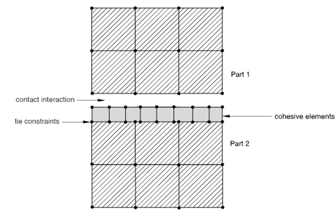
Figure 10: Contact interaction on one side of a cohesive zone

There are three examples in this tutorial “Implementation of Cohesive by interaction & element based methods in ABAQUS” :

4. Defining the cohesive element’s initial geometry

The initial geometry of a cohesive element is defined:

• by the nodal connectivity of the element and the position of these nodes;
• by the stack direction, which can be used to specify the top and the bottom faces of the cohesive element independent of the nodal connectivity; and
• by the magnitude of the initial constitutive thickness, which can either correspond to the geometric thickness implied by the nodal positions and stack direction or be specified directly.

4.1. Defining the element connectivity

The connectivity of a cohesive element is like that of a continuum element; however, it is useful to think of a cohesive element as being composed of two faces (a bottom and a top face) separated by the cohesive zone thickness. The element has nodes on its bottom face and corresponding nodes on its top face. Pore pressure cohesive elements include a third, middle face, which is used to model fluid flow within the element.

Three methods are available to define the element connectivity:

1. By directly defining the element’s complete connectivity

The complete connectivity of a cohesive element can be given directly.

2. By defining the bottom-face element connectivity and an integer offset

Alternatively, you can specify the connectivity of the bottom face plus a positive integer offset that will be used to determine the remaining cohesive element nodes.

3. By defining the bottom- and top-face element connectivities and an integer offset

When you define the bottom and top face nodes, the integer offset will be used to define the node numbers of the middle face, with the numbering of the middle-face nodes offset from the bottom face node numbers.

4.2. Specifying the constitutive thickness

You can specify the constitutive thickness of the cohesive element directly or allow Abaqus to compute it based on nodal coordinates such that the constitutive thickness is equal to the geometric thickness. The default behavior depends on the nature of the application.

If the geometric thickness of the cohesive element is very small compared to its surface dimensions, the thickness computed from the nodal coordinates may be inaccurate. In such cases, you can specify a constant thickness directly when defining the section properties of these elements. The characteristic element length of a cohesive element is equal to its constitutive thickness.

• When the response of the cohesive elements is based on a continuum approach, by default the constitutive thickness of the element is computed by Abaqus based on the nodal coordinates. You can override this default by specifying the constitutive thickness directly:

Property module: cohesive section editor: Response: Continuum: Initial thickness: Use nodal coordinates, Specify: thickness, or Use analysis default (Figure 11).

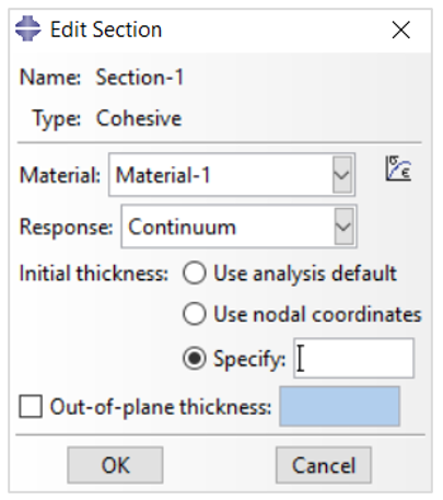
Figure 11: Defining cohesive element constitutive thickness

• When the response of the cohesive elements is based on a traction-separation approach, Abaqus assumes by default that the constitutive thickness is equal to one. This default value is motivated by the fact that the geometric thickness of cohesive elements is often equal to (or very close to) zero for the kinds of applications in which a traction-separation-based constitutive response is appropriate. You can override this default by specifying another value or specifying that the constitutive thickness should be equal to the geometric thickness.

Property module: cohesive section editor: Response: Traction Separation: Initial thickness: Specify: thickness, Use analysis default, or Use nodal coordinates

• When the response of the cohesive elements is based on a uniaxial stress state, there is no default method for computing the constitutive thickness. You must indicate your choice of the method of determining the constitutive thickness.

Property module: cohesive section editor: Response: Gasket: Initial thickness: Specify: thickness or Use nodal coordinates

It is important to define the orientation of cohesive elements correctly since the behavior of the elements is different in the thickness and in-plane directions. By default, the top and bottom faces of cohesive elements are as shown in figure 12 for three-dimensional cohesive elements and figure 13 for two-dimensional and axisymmetric cohesive elements.

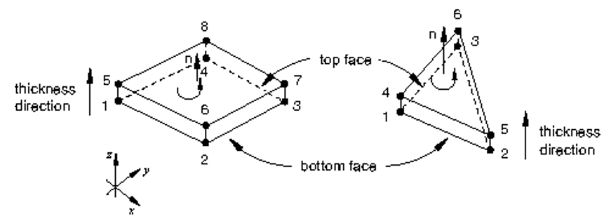
Figure 12: Default thickness direction for three-dimensional cohesive elements

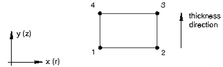
Figure 13: Default thickness direction for two-dimensional and axisymmetric cohesive elements

4.3. Setting the stack direction equal to an isoparametric direction

The “stack direction” refers to the isoparametric direction along which the top and bottom faces of a cohesive element are stacked. By default, the top and bottom faces are stacked along the third isoparametric direction in three-dimensional cohesive elements and along the second isoparametric direction in two-dimensional and axisymmetric cohesive elements. The choice of the isoparametric direction depends on the element connectivity.

You cannot define the stack direction based on isoparametric directions in Abaqus/CAE. The stack direction will correspond to the default discussed earlier. The isoparametric direction choices for three-dimensional cohesive elements are shown in figure 14.

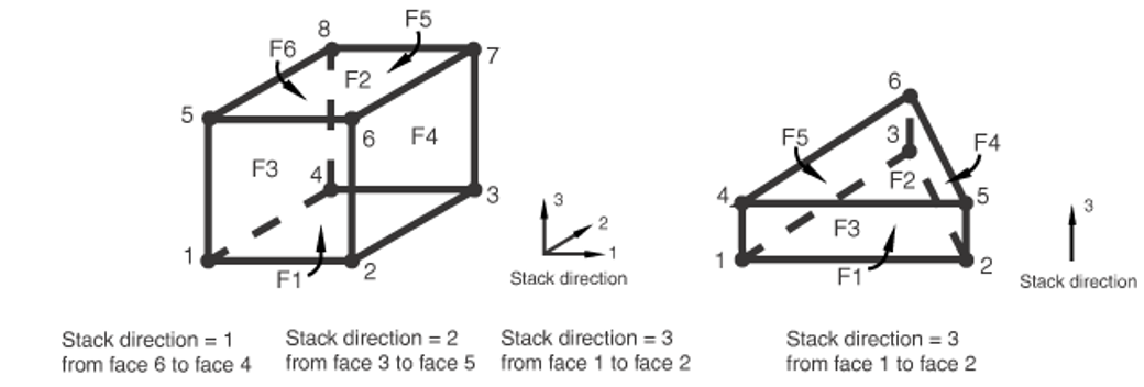
Figure 14: Stack directions for COH3D8 (left) and COH3D6 (right) elements

At this point, we finish our discussion about cohesive elements in Abaqus and summarize what we talked about in this article.

5. Abaqus Cohesive Behavior

In Abaqus you can also define cohesive contact where two parts of your model connected together using cohesive material (Abaqus cohesive contact). This modeling in Abaqus is known as Surface-based Cohesive Behavior.

5.1. Surface-based Cohesive Behavior

Surface-based cohesive behavior provides a simplified way to model cohesive connections with negligibly small interface thicknesses using the traction-separation constitutive model. It can also model “sticky” contact (surfaces can bond after coming into contact).

The cohesive surface behavior can be defined for general contact in Abaqus/Explicit and contact pairs in Abaqus/Standard (with the exception of the finite-sliding, surface to-surface formulation). Cohesive surface behavior is defined as a surface interaction property (Figure 15).

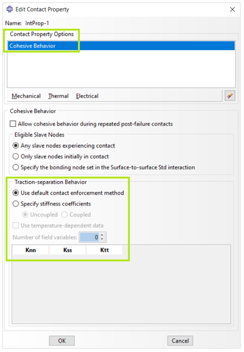
Figure 15: Defining cohesive contact property in Abaqus

Now let’s compare the cohesive elements and cohesive surfaces in Abaqus.

5.2. Element- vs Surface-based Cohesive Behavior

Cohesive elements:

• Must be bonded at the start of the analysis.
• Once the interface has failed, the surfaces do not re-bond.
• Allow for several constitutive behavior types including: Traction-separation constitutive model, Continuum-based constitutive model and Uniaxial stress-based constitutive model.
• The element material definitions include mass.
• Are recommended for more detailed adhesive connection modeling.

Cohesive surfaces:

• Can bond anytime contact is established (i.e., “sticky” contact behavior); So, Cohesive interface need not be bonded at the start of the analysis.
• You can control whether debonded surfaces will stick or not stick if contact occurs again. By default, they do not stick.
• Must use the traction-separation interface behavior.
• Do not add mass to the model. Indented for thin adhesive interfaces; thus, neglecting adhesive mass is appropriate for most applications.
• Provides a quick and easy way to model adhesive connections

At this point, we finish our discussion about cohesive elements in Abaqus and summarize what we talked about in this article.

6. Summary

We started our discussion with the definition and importance of cohesive elements. Some of their application also introduced. Three different responses to the applied load in cohesive elements were discussed briefly. The Abaqus cohesive elements’ library introduced.  Then we went through the modeling of cohesive zones and different types of connection between cohesive layer and the neighbor components. Then, we talked about the cohesive elements’ initial geometry. At the final section, we introduced Abaqus cohesive behavior and Abaqus cohesive contact. We compared the cohesive element modeling and cohesive contact modeling so you can decide better to implement which one in your analysis.

This article is an introduction to cohesive elements modeling and aims to clarify the initial concepts you need to know in order to model cohesive zones in your Abaqus analyses.

In the end, we appreciate for reading this article. Don’t forget to leave us your comments about this article to improve our content quality. Wish you the Best.

One last note:

Did you know that when it comes to simulating the separation of bonded materials, Abaqus offers two key approaches: cohesive elements and cohesive interaction?

Cohesive interaction is a surface-based approach. It defines a traction-separation relationship directly between contacting surfaces. This simplifies the model setup compared to cohesive elements, making it ideal for situations where the adhesive layer is thin or its detailed behavior is less critical.

But these info just basics; you can learn more just by watching the tutorial below:

This package teaches you how to choose the method and apply cohesive modeling for various simple and complex problems. The training package also teaches you how to define the basic geometry of the adhesive elements and how to define the mechanical behavior in elastic and damaged regions in ABAQUS FEM software.

It would be helpful to see Abaqus Documentation to understand how it would be hard to start an Abaqus simulation without any Abaqus tutorial.