
Abaqus DFLUX & VDFLUX FREE Tutorial: Step by Step Guide

Did you know that in the real world, heat transfer and mass diffusion often occur unevenly? From electronic devices where some parts heat up faster to industrial processes like welding with highly localized heat sources, nonuniform fluxes play a critical role in accurately modeling these phenomena.
The DFLUX and VDFLUX subroutines in Abaqus allow engineers to define such nonuniform heat or mass flux distributions. Unlike standard options (e.g. Abaqus GUI), these subroutines provide flexibility to incorporate complex dependencies on variables like time, position, temperature, and material properties. Whether for simulating heat generation in electronics or mass transfer in diffusion processes, DFLUX is indispensable for capturing realistic conditions in simulations.
This tutorial explores the key aspects of the DFLUX VDFLUX subroutines in Abaqus, including their structure, variables, and implementation steps. You’ll also learn about real-world applications like arc welding and laser welding, along with practical examples and tips for effective use. By the end of this blog, you’ll have a clear understanding of how DFLUX can enhance your simulation accuracy.
The DFLUX and VDFLUX subroutines in Abaqus allow for the definition of spatially and temporally varying fluxes in heat transfer simulations. In this tutorial package, you will learn how to implement these subroutines for different types of thermal loads, including uniform, radially symmetric, and time-dependent fluxes, as well as apply them to complex heat transfer problems such as welding simulations.
 |
|
1. What is Abaqus DFLUX subroutine?
The DFLUX subroutine in Abaqus is a user-defined subroutine that allows users to define nonuniform distributed fluxes for heat transfer or mass diffusion analyses. It provides a way to control the magnitude and distribution of flux (such as heat flow or mass flow) as a function of variables like position, time, temperature, and element properties. This subroutine offers flexibility to account for complex, real-world conditions that cannot be captured using standard Abaqus input options. It overrides the default uniform flux input in Abaqus, enabling users to introduce more realistic thermal or mass diffusion boundary conditions.
1.1. When Should We Use the DFLUX Subroutine?
The DFLUX subroutine should be used when a nonuniform flux distribution is required. It is particularly valuable when the flux depends on complex factors that change over time, space, or with certain material behaviors.
Here are the key scenarios where the DFLUX subroutine is essential:
- Heat Transfer Problems:
- To apply a nonuniform heat flux in models where heat is not uniformly distributed.
- Example: In electronic devices, heat generation varies across components due to different material properties and power consumption.
- Mass Diffusion Problems:
- To model nonuniform mass flux in diffusion processes where the mass transfer rate varies across surfaces or within materials.
- Example: A sugar cube added to a cup of coffee dissolves nonuniform but eventually diffuses to make the concentration uniform.
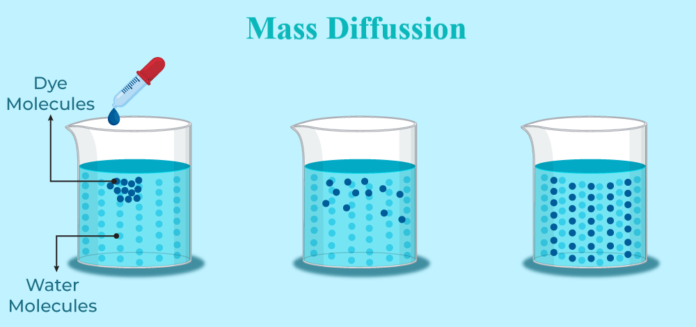
Figure 1: Mass diffusion process example [Ref]
- Time-Dependent Flux:
- In transient analyses, where the flux changes over time. The DFLUX subroutine allows users to specify time-varying flux patterns.
- Example: Simulating heat flux from a cup of hot coffee. The heat flux to the surrounding air decreases over time as the coffee cools.
- Flux Dependent on Position or Material Properties:
- The subroutine can incorporate complex relationships between position, material properties, and boundary conditions.
- Example: Heat flux on a car’s hood after driving. The flux is stronger near the engine compartment and weaker near the sides of the hood.
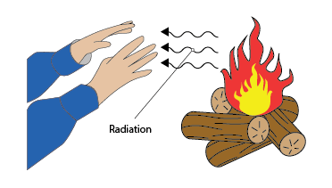
Figure 2: radiative heat flux that can vary with distance from the fire [Ref]
So, the DFLUX subroutine in Abaqus is a powerful tool for simulating real-world thermal and diffusion processes where nonuniform fluxes are involved. It enables users to model complex boundary conditions that cannot be captured using standard inputs, making it essential for accurate simulations in fields like electronics, aerospace, manufacturing, and chemical engineering.
2. Abaqus DFLUX subroutine interface and variables
The DFLUX subroutine is written in Fortran and is used in Abaqus/Standard to define nonuniform distributed fluxes. It is called at each flux integration point during the analysis and allows users to control the flux as a function of position, time, and other variables.
If you do not anything about the Fortran do not worry! We’ve got you covered with this blog: “Abaqus Fortran “Must-Knows” for Writing Subroutines“.
In this section, we’ll cover:
- DFLUX subroutine interface.
- DFLUX subroutine variables.
- Step-by-step Implementation of DFLUX subroutine in Abaqus.
2.1. DFLUX Subroutine Interface
Abaqus software has defined a specific structure and variables for each subroutine, so users must follow these coding structures to use these subroutines. You can see the DFLUX subroutine interface introduced by Abaqus in the figure below.
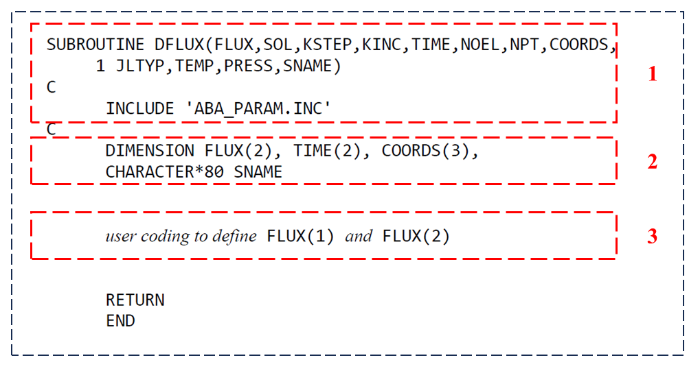
Figure 3: DFLUX subroutine interface
As you can see, this subroutine, like other subroutines, has three general sections. The first section is about introducing the variables that are used in this subroutine. The second section is about determining the dimensions of the variables, and the third section is where the user must determine the flux conditions.
The key task for the user is to define the magnitude of the flux (stored in the FLUX array) based on input variables such as the element number, integration point, temperature, and coordinates.
2.2. DFLUX Subroutine Variables
As mentioned, there are various variables used in the DFLUX subroutine. Each of these variables is defined by Abaqus for a specific application. Below is a detailed explanation of all the variables in the DFLUX subroutine:
|
Variable |
Type | Description |
| FLUX(1) | To be defined |
Magnitude of the flux flowing into the model at point. For heat transfer, units are JT⁻¹L⁻² (surface flux) or JT⁻¹L⁻³ (body flux). In mass diffusion cases the units are PLT⁻¹ for surface fluxes and PT⁻¹ for body flux. In transient analyses, FLUX(1) must be defined as the time average flux over the time increment, not the instantaneous value at the end of the time increment. This is crucial for accurate energy balance in time-dependent problems. |
| FLUX(2) | To be defined |
The rate of change of the flux with respect to the temperature (heat transfer) or concentration (mass diffusion) at the point. For heat transfer, units are JT⁻¹L⁻²K⁻¹ (surface flux) or JT⁻¹L⁻³K⁻¹ (body flux). Defining FLUX(2) helps improve convergence during nonlinear solution processes, especially when the flux is strongly temperature-dependent. |
| KSTEP | Passed in for information |
Current step number in the analysis. Allows the user to apply different flux conditions depending on the step. Useful for multi-step simulations with varying boundary conditions. |
| TIME(1) | Passed in for information |
Represents the elapsed time in the current step (Current step time). Useful for defining time-dependent fluxes, such as a heat flux that increases linearly or exponentially during the step. |
| TIME(2) | Passed in for information |
Represents the cumulative time from the start of the simulation (Total time elapsed). This is helpful for defining fluxes that depend on the entire simulation timeline, not just the current step time. |
|
COORDS(3) |
Passed in for information |
Coordinates of the current integration point. If geometric nonlinearity is considered, these are the current coordinates; otherwise, they are the initial coordinates. Useful for applying spatially varying fluxes, such as Gaussian heat sources or position-dependent mass diffusion. |
| TEMP | Passed in for information |
Current temperature at the integration point (used for mass diffusion problems). For heat transfer problems, temperature is passed as SOL variable. Useful for applying temperature-dependent boundary conditions in diffusion analyses. |
There are other variables such SNAME, PRESS, JLTYP, NPT, NOEL, SOL, and KINC and all of them are for in for information variables. These variables can be used to calculate variables that should be defined. Additional explanations about these and other variables in the DFLUX subroutine can be found in the “DFLUX Subroutine (VDFLUX Subroutine) in ABAQUS” package from the caeassistant team.
2.3. Step-by-step Implementation of DFLUX subroutine in Abaqus
Using the DFLUX subroutine in Abaqus can be challenging. To implement this subroutine in Abaqus, the user must go through the following steps:
- Creating a suitable simulation model such as creating parts, steps, meshes, etc. in the Abaqus graphical user interface (GUI)
- Writing and preparing the DFLUX subroutine in the format specified by Abaqus
- Introducing the subroutine to Abaqus and linking it to the created model.
To use the DFLUX subroutine, a standard solver and the appropriate step must be used. You can see the steps that DFLUX and VDFLUX are in:
- DFLUX:
- Heat transfer step
- Mass diffusion step.
- VDFLUX:
- Coupled step
- temp-displacement step
- Coupled thermal-electric step
- Coupled thermal-electrical-structural step
- Dynamic, Temp-disp, Explicit step
the most important variables of the DFLUX subroutine are fully explained in our tutorial with three simple questions:
For example, the DFLUX subroutine can be used in the heat transfer step. As you can see in the next figure, only the Thermal category and different heat flux types are available for loading in the heat transfer step.
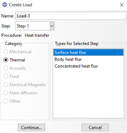
Figure 4: Load module in heat transfer step
The next step to use the DFLUX subroutine is to set the Distribution option to User-Defined. This means you specify the heat transfer value according to the subroutine. You should also note that the value you specify for Magnitude is multiplied by the output value of the subroutine. So, by setting this value equal to one, the output value of the subroutine will not change.
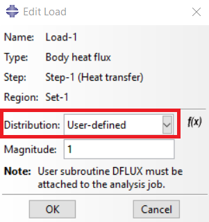
Figure 5: Applying DFLUX subroutine as user-defined distribution
One of the important points in using thermal analysis is to determine the absolute zero temperature. To do this, we must determine the value in the Edit Model Attribute window. Note that if you are using Celsius temperature units, you must determine the absolute zero temperature equal to -273.15. Also, if radiation will occur in your model, you must also determine the Stefan-Boltzmann constant.
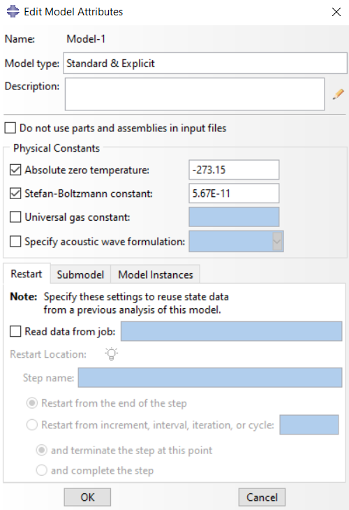
Figure 6: Determining absolute zero temperature and Stefan-Boltzmann constant
3. When to Use What is Abaqus VDFLUX Subroutine and when to use it?
Abaqus provides two different subroutines to define nonuniform flux boundary conditions for heat transfer and mass diffusion problems:
- DFLUX (for use in Abaqus/Standard)
- VDFLUX (for use in Abaqus/Explicit)
While DFLUX handles flux definitions in static or transient heat transfer and mass diffusion problems, the VDFLUX subroutine is used in Abaqus/Explicit to define nonuniform distributed fluxes in dynamic coupled temperature-displacement analyses. Unlike DFLUX, which works in Abaqus/Standard, VDFLUX is specifically designed for explicit integration schemes where both temperature and structural responses are solved together.
VDFLUX is used when dealing with explicit dynamic problems where the applied flux varies with:
- Position (spatial coordinates)
- Temperature
- Time
- Velocity of the material
- Orientation of the element face or edge
We mentioned that in the DFLUX we can define Fluxes dependent on time, position, and temperature, right? the VDFLUX has all plus Velocity dependences as well! Moreover, in this tutorial we tell you ” How to convert DFLUX to VDFLUX and vice versa? “
Examples of problems where VDFLUX is used:
- Thermal shock during high-speed impacts
- Heat generation due to friction or deformation in crash simulations
- Explosive heating scenarios in materials
3.1. VDFLUX subroutine Interface
The VDFLUX subroutine interface is slightly different from DFLUX, as it is designed to handle multiple points simultaneously. Like the DFLUX subroutine, this subroutine also has a format specified by Abaqus and has three general sections. Here’s the basic structure of the VDFLUX subroutine:
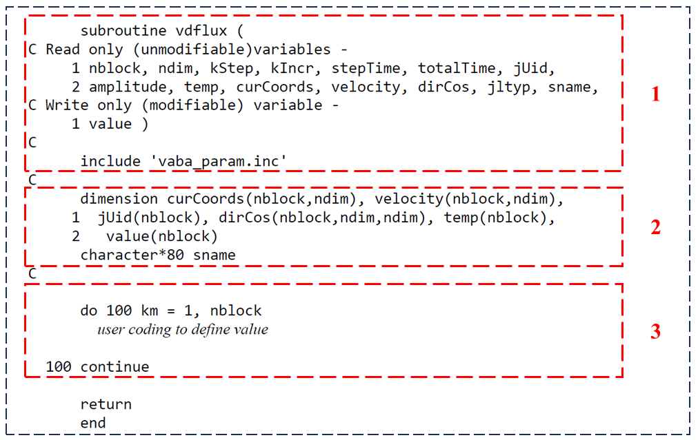
Figure 7: VDFLUX subroutine interface
3.2. VDFLUX subroutine Variables
The VDFLUX subroutine also has variables, some of which are shared with the DFLUX subroutine, and some are specific to this subroutine. Below is a detailed explanation of all the variables passed to the VDFLUX subroutine:
| Variable | Type | Description |
|
value(nblock) |
To be defined |
The flux magnitude at each point being processed. This must be calculated by the user for all points in the current call. Units depend on the analysis type: JT⁻¹L⁻² for surface fluxes and JT⁻¹L⁻³ for body fluxes. |
| nblock | Passed in for information |
The number of points being processed in the current subroutine call. Allows simultaneous evaluation of flux at multiple points. |
| stepTime | Passed in for information |
The time elapsed within the current step. Helps define time-dependent fluxes for transient conditions. |
|
totalTime |
Passed in for information |
The total time elapsed since the start of the simulation. Useful for global time-dependent fluxes across multiple steps. |
|
temp(nblock) |
Passed in for information |
The current temperature at each flux point. This variable is critical for defining fluxes that depend on temperature. |
|
curCoords(nblock, ndim) |
Passed in for information |
The current spatial coordinates of each point being processed. Enables position-dependent flux calculations. |
|
dirCos(nblock, ndim, ndim) |
Passed in for information |
The direction cosines define the orientation of the surface or edge where the flux is applied. Helps handle flux directions for both 2D and 3D elements. |
|
velocity(nblock, ndim) |
Passed in for information |
The current velocity at each point. Used in fluxes that depend on the motion of the material or boundary. |
Like the table of DFLUX subroutine variables, this table also does not mention a number of variables (ndim, kStep, kIncr, jUid, amplitude, jltyp, and sname) that you can use the “DFLUX Subroutine (VDFLUX Subroutine) in ABAQUS” package to learn more about.
Before we go any further, if you consider yourself new in the Abaqus subroutine, we have a blog about it and you can learn the basic stuff about it: “Abaqus subroutine“.
4. DFLUX VS VDFLUX
In general, you can see the differences between the two subroutines, DFLUX and VDFLUX, as summarized in the table below.
| Aspect | DFLUX | VDFLUX |
| Solver |
Abaqus/Standard |
Abaqus/Explicit |
|
Analysis Type |
Static or transient heat transfer, mass diffusion |
Dynamic coupled temperature-displacement |
|
Key Variable to Define |
FLUX(1), FLUX(2) |
value(nblock) |
|
Flux Dependencies |
Position, time, temperature |
Position, time, temperature, velocity |
Remember that some of the variables in the VDFLUX subroutine are Equivalent to the variables in the DFLUX subroutine. The table below shows these variables and their equivalents.
|
DFLUX variables |
VDFLUX equivalent variables |
|
FLUX(1) |
value |
|
TIME(1) |
stepTime |
|
TIME(2) |
totalTime |
| COORDS | curCoords |
| SNAME | sname |
| JLTYP | jltyp |
| KSTEP | kStep |
| KINC | kIncr |
| SOL | temp |
5. DFLUX and VDFLUX applications
As mentioned earlier, the DFLUX and VDFLUX subroutines can simulate real-world heat transfer for users. Here are a few engineering and real-world processes that these subroutines can help with in the simulation process:
| Process | Description | Subroutine |
| Arc Welding | Simulates a moving arc heat source with nonuniform heat flux | DFLUX |
| Laser Welding | Models concentrated laser energy input with a Gaussian heat distribution | DFLUX |
| Moving Heat Sources | Heat sources that move across the material surface during the simulation | DFLUX/VDFLUX |
| Friction Stir Welding | Applies heat generated by friction between rotating tools and the material | DFLUX |
| Induction Heating | Simulates electromagnetic heat generation within a material | VDFLUX |
| Explosive Heating | Models rapid heat generation in materials due to explosive events | VDFLUX |
- Moving Heat Source Models: Goldak’s Double-Ellipsoidal Heat Source Model
There are various models to determine the heat transfer distribution that can be used in the DFLUX and VDFLUX subroutines. Models such as Goldak, Gaussian model, etc. One of the most popular models for simulating arc welding processes is Goldak’s model, which uses a double-ellipsoidal heat distribution to represent the heat flux in both the front and rear halves of the weld pool. Goldak’s model is widely used because it provides a more accurate representation of the weld pool compared to simpler models. The heat flux in Goldak’s model is defined as:
-
- Front Half:
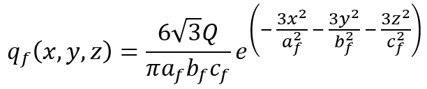
-
- Rear Half:
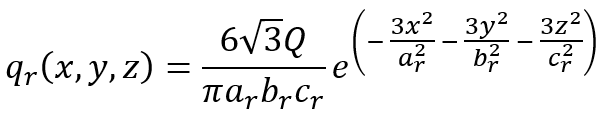
Where:
- q = heat distribution
- x, y, z = Current position
- Q = Total heat input
- a, b, c = Dimensions of the ellipsoid in the x, y, and z directions
- r and f represent rear and front respectively
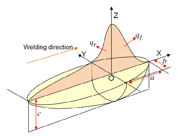
Figure 8: Goldak’s double ellipsoidal heat source model diagram [Ref]
- Gaussian Heat Source Model
The Gaussian heat source model is a commonly used approach to represent concentrated heat sources like lasers or electron beams. It is based on the Gaussian distribution, which describes how heat intensity is highest at the center of the heat source and decreases radially outward. This model is ideal for processes like laser welding, laser heating, and focused energy beam applications.
The 2D Gaussian heat source is described by the following equation:
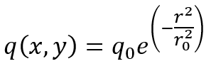
Where:
- q(x, y): Heat flux at a point(x, y);
- q0: Maximum heat flux at the center of the heat source;
- r: Radial distance from the center of the heat source.
![]()
- (x0 , y0): Are the coordinates of the heat source center.
- r0 : Standard deviation of the heat source (that determines how far the heat spreads).
In the 3D Gaussian model r is defined as:
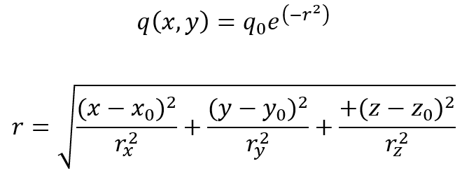
- rx, ry, rz: Characteristic decay radii in the x, y, and z directions, respectively.
Now let’s examine some of these subroutine examples.
5.1. Arc Welding using DFLUX subroutine (3D body flux)
The first step in simulation using the DFLUX subroutine is modeling in the Part module. The figure below shows a model created for welding two sheets in the Part module, in which the path of the heat source is also specified. We have another arc welding simulation with full tutorial and subroutine codes in the second workshop of the DFLUX and VDFLUX tutorial package.
Also, if you are interested to know all about welding and Abaqus welding simulation, read this blog: “Abaqus Welding Simulation Complete Guide: Essential Methods and Theories Explained“
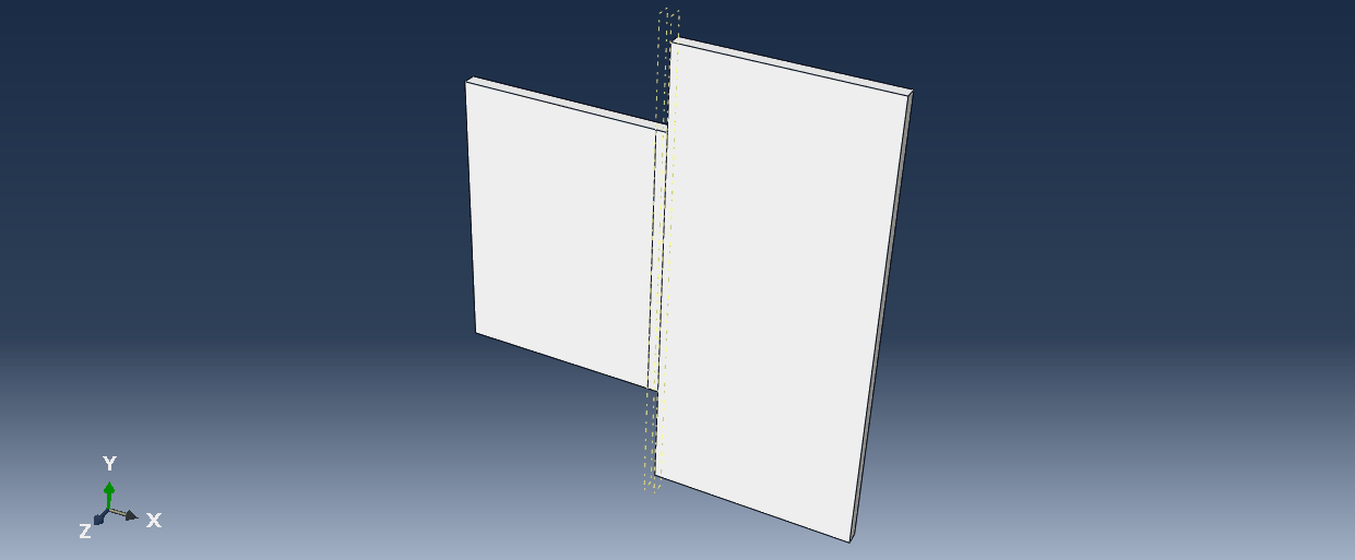
Figure 9: Model created in the Part module
The next step is to assign the thermal properties required for the welding simulation. The figure below shows the created material and its thermal properties.
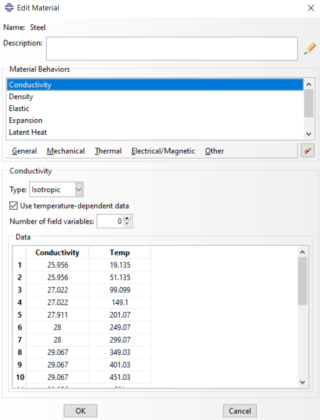
Figure 10: Property module
After assigning the materials, it is time to create the appropriate steps. For welding, the heat transfer step should be used. The important point in this module is to create the welding and cooling steps separately. The cooling module requires several times more time. In this module, users must specify the maximum temperature increase in each increment as shown in the figure below.
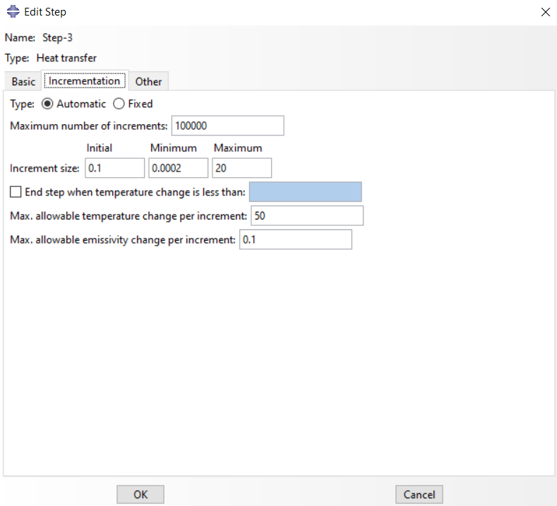
Figure 11: Maximum allowable temperature change per increment
And finally, it is time to apply thermal force to the sheets. As mentioned earlier, in this module, by selecting the user-defined distribution, the subroutine takes over the task of distributing heat on the model.
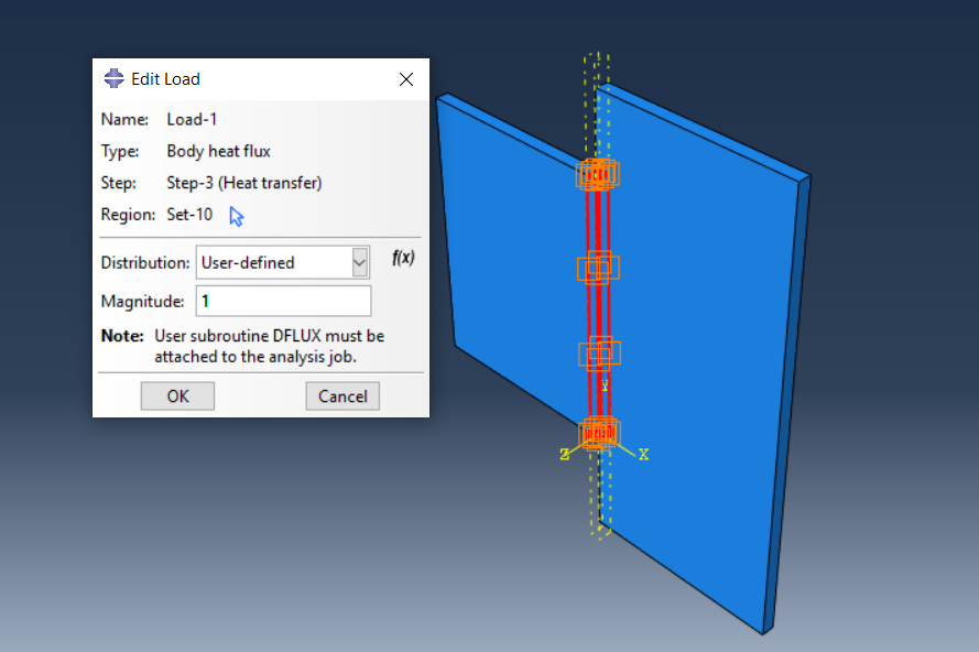
Figure 12: Applying heat to sheets by DFLUX subroutine
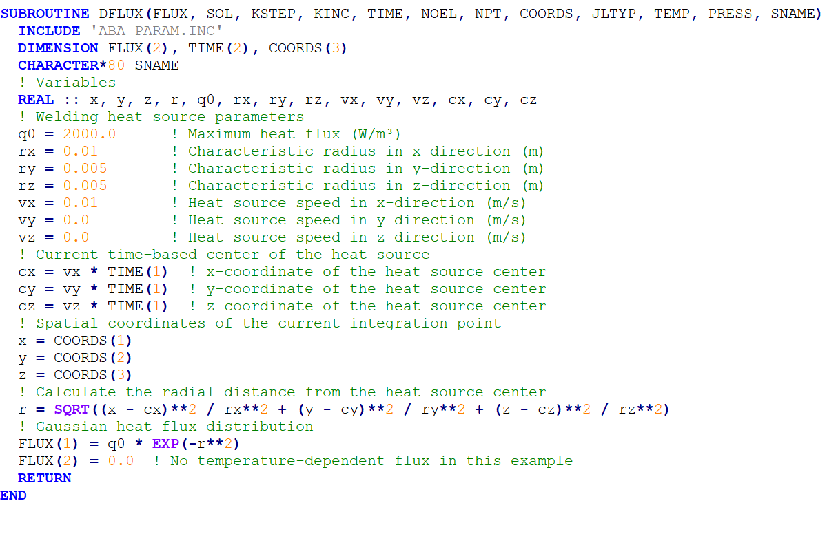
Figure 13: Arc Welding DFLUX subroutine
As you can see, in this subroutine, the FLUX(1) is calculated as “to be defined” variable. This subroutine is a 3D heat distribution, so the COORDS variable has three components. In this heat distribution, a 3D Gaussian model is used. Note that the heat source center position is calculated by multiplying the heat source’s speed (![]() ) by time (TIME(1)). Here you can see the welding simulation using the DFLUX subroutine.
) by time (TIME(1)). Here you can see the welding simulation using the DFLUX subroutine.
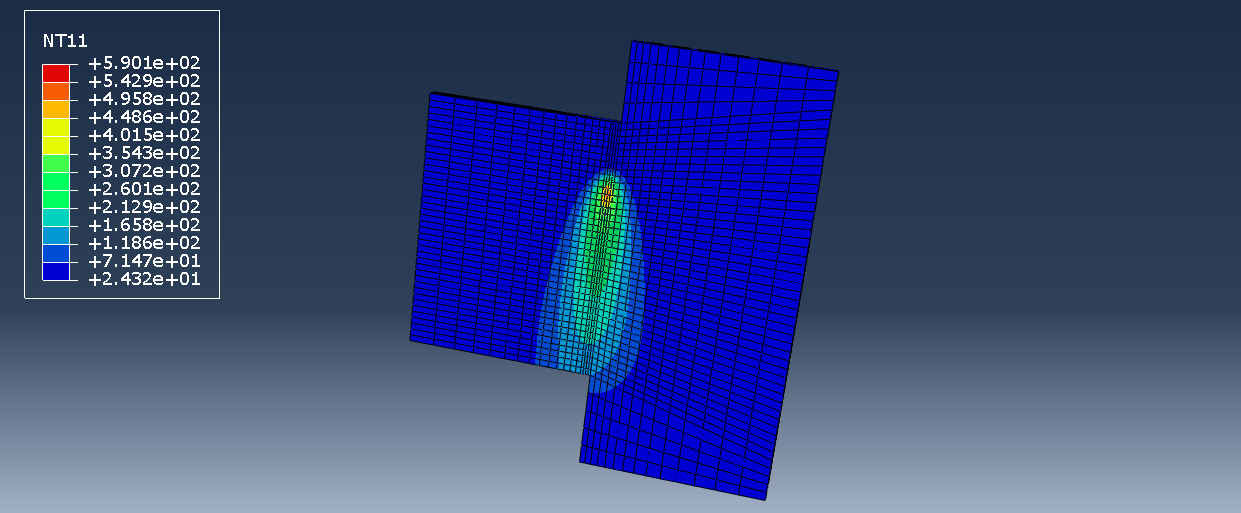
Figure 14: Temperature distribution during the welding process
5.2. Laser Welding DFLUX subroutine (2D Surface Flux)
In the laser welding example, the DFLUX subroutine, unlike the previous example, is considered 2D, so the variable COORDS (the input variable of the laser beam position) has 2 components. As in the previous example, the purpose of this subroutine is to determine the value of the FLUX(1).
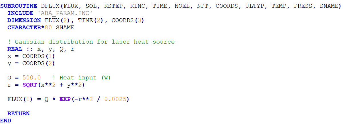
Figure 15: Laser Welding DFLUX subroutine
The DFLUX and VDFLUX subroutines in Abaqus allow for the definition of spatially and temporally varying fluxes in heat transfer simulations. In this tutorial package, you will learn how to implement these subroutines for different types of thermal loads, including uniform, radially symmetric, and time-dependent fluxes, as well as apply them to complex heat transfer problems such as welding simulations.
|
|
6. Conclusion
In this article, we explored the DFLUX and VDFLUX subroutines in Abaqus, user-defined tools for applying nonuniform heat flux and mass diffusion in heat transfer and diffusion analyses. This capability is crucial for modeling realistic scenarios where flux distributions depend on factors like time, position, and material properties.
We began by explaining what the DFLUX subroutine is and when it should be used, highlighting its flexibility in handling complex flux patterns. Next, we detailed its interface and variables, showing how to implement it step by step. We also discussed the differences between DFLUX and VDFLUX subroutines and provided examples of their applications in processes like welding.
Overall, we learned how DFLUX enables more accurate simulations of thermal and diffusion processes, especially in cases with nonuniform conditions. This tool is essential for engineers working on simulations that require precision and adaptability beyond standard options in Abaqus.