
Abaqus load types: Applying loads in Abaqus
How should we apply loading to an Abaqus model? When simulating in Abaqus, it is important to understand how to apply the appropriate types of loads. Loads in Abaqus represent forces, stresses, or constraints that directly affect how your model behaves. Correct application of these loads ensures that the analysis results are as accurate and reliable as possible.
The type of Abaqus load that you apply to your model will depend on the specific problem that you are trying to solve. For example, if you are trying to simulate the stress in a beam under a point load, you would apply a point load to the beam. For instance, applying a pressure load instead of a concentrated force can change the stress distribution in a structure. This could lead to results that do not represent the actual scenario, potentially causing safety issues or design failures in real-world applications. Therefore, knowing how to apply different load types in Abaqus is key to ensuring valid results.
In this article, we’ll explore the various Abaqus load types, including mechanical, thermal, and more. We will look at how to apply these loads effectively within your simulations, from concentrated forces to distributed pressures, and discuss how load amplitudes influence the analysis.
1. Applying Abaqus Load
Abaqus load application is crucial for accurate and reliable finite element analysis results in Abaqus. In Abaqus, loads are applied to models to simulate real-world physical forces and constraints that affect a model’s behavior under various conditions. These loads can be applied as forces, pressures, temperatures, or displacements across different steps, representing various stages in an analysis. Abaqus offers flexibility with load types, including mechanical, thermal, and boundary conditions, all essential for capturing a realistic response from the model.
Why Correctly Determining the Type of Loading is Important: Accurate load determination is critical in finite element analysis (FEA) because the results directly depend on how loads are applied. Incorrect loading can lead to unrealistic results, which may cause design failures, safety risks, or costly errors in real-world applications. For example, applying a pressure load instead of a concentrated force load could change the stress distribution in a structure, leading to misleading outcomes.
Abaqus allows you to apply loads through its Graphical User Interface (GUI) or scripting using Python. Users can define loads within the model’s assembly, directly on geometry. The application of loads can be step-dependent, which means different loads can be applied in different stages of the analysis. This capability is crucial for simulating complex, real-world scenarios where the conditions change over time.
According to the explanations that were given about the importance of loading in Abaqus software, now it is better to review some of the loading types in Abaqus software.
2. What are Abaqus load types?
In Abaqus, load categories are broad classifications that represent different types of physical phenomena affecting a model. These categories include mechanical loads (e.g., forces, pressures, moments), thermal loads (e.g., temperatures, heat fluxes), fluid loads, and mass diffusion loads. Each category contains specific Abaqus load types that describe how the load is applied, such as concentrated forces, distributed pressures, or body forces. These load types define how forces and conditions act on the model during analysis. Figure 1 shows load categories and Abaqus load types when generating forces in Abaqus.
In the following sections, we will examine each load category and its associated load types in more detail.
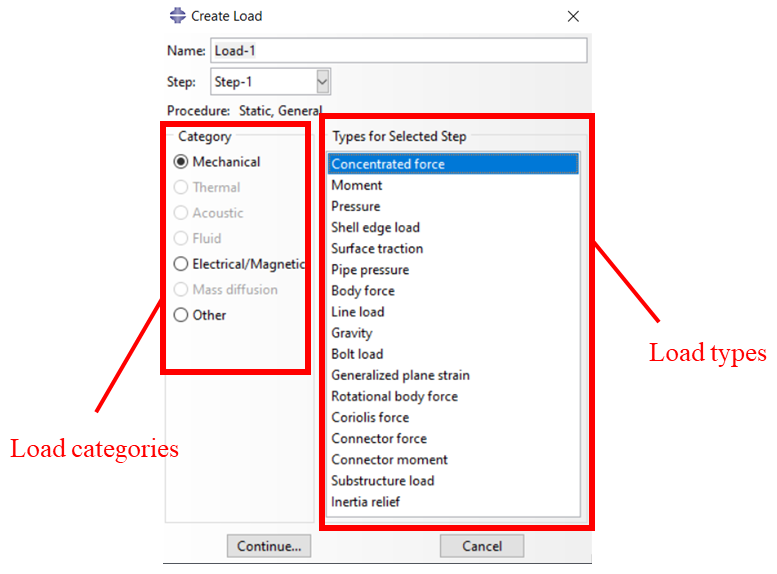
Figure 1: Load categories and Abaqus Load types in create load dialog box
2.1. Mechanical Loads
Mechanical loads in Abaqus represent physical forces or actions applied to a structure, affecting its behavior under different conditions. These include forces, pressures, and moments applied to structures. They simulate real-world conditions like weight, wind pressure, or external forces acting on an object. In general, mechanical loads can be divided into two categories:
- Concentrated loads: These loads are applied at specific points within the model. They represent forces or moments that are concentrated at a particular location. Like a single point force acting on the center of a beam.
- Distributed loads: This type of load is spread over a surface area or volume of the model. It simulates forces that are applied over a continuous region. Common examples include pressure, and gravity acting on the volume of a structure.
Now we will examine some types of mechanical loading in detail:
2.1.1. Concentrated Force
Concentrated Force is a force applied at a specific point on the model. It is typically used in structural analysis where a load is concentrated at a small area, such as a load on a beam’s tip. It is crucial for modeling scenarios where loads are concentrated.
To create a “Concentrated Force” in Abaqus using the Load Module, in the “Create Load” dialog box, select “Mechanical” and choose “Concentrated Force” as the load type. You can learn this type of load in a practical example 2D truss modeling.
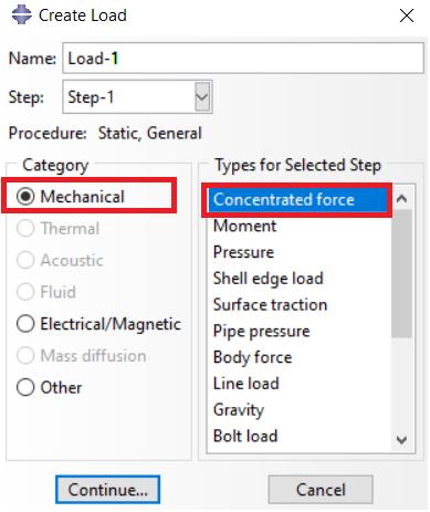
Figure 2: Creating Concentrated Force
Then choose the point or node where you want to apply the force and specify the magnitude and direction of the force in the load editor dialog box.
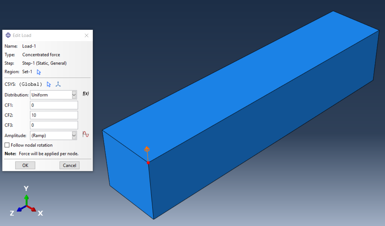
Figure 3: Selected point and magnitude of the force in different directions
| If you need deep training, our Abaqus Course offerings have you covered. Visit our Abaqus course today to find the perfect course for your needs and take your Abaqus knowledge to the next level! |
 |
In this Abaqus training package for beginners, which is designed for FEM Simulation students in mechanical engineering, various examples in the most widely used fields are presented:
|
2.1.2. Abaqus Pressure Load
Abaqus Pressure Load is a Abaqus distributed load acting perpendicular to a surface. It is commonly used for simulating fluid pressure on walls, such as water pressure on a dam.
To create a “Pressure Load” in Abaqus, after choosing “Mechanical” and selecting “Pressure” in the “Create Load” dialog box as the load type, pick the surface or face where the pressure will be applied. Then specify the pressure magnitude (positive or negative) in the load editor (Figure 5).
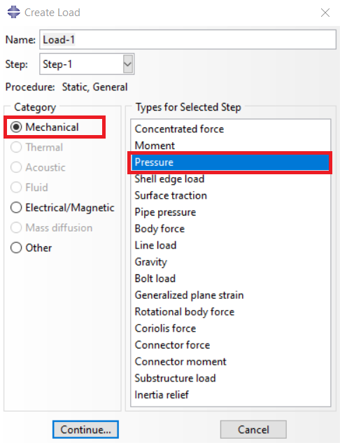
Figure 4: Creating Pressure Load
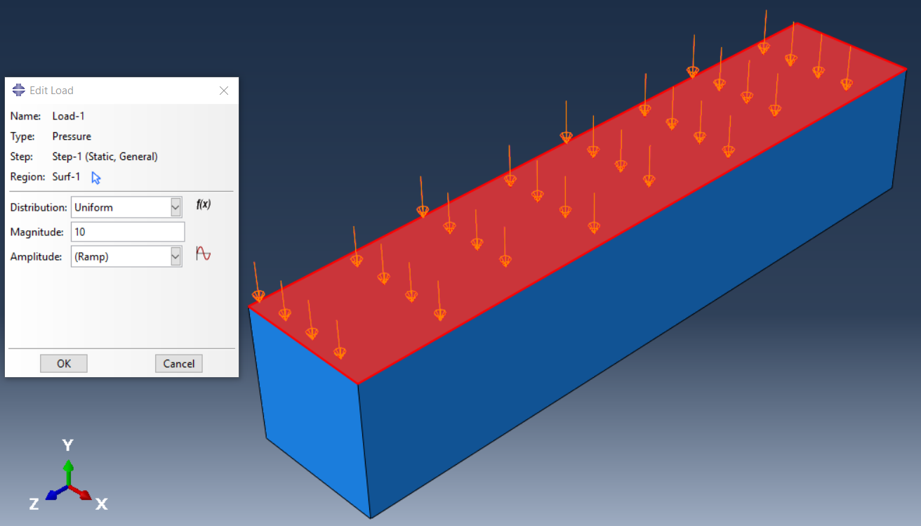
Figure 5: Selected surface and magnitude of the Pressure
2.1.3. Surface Traction
Surface Traction is a force distributed over a surface that can act in any direction, simulating loads such as frictional forces on a contact surface.
To create a Surface Traction Force in Abaqus, after choosing “Surface Traction” as the load type and picking the surface where the traction force will be applied, you must Specify the traction force magnitude and direction in the load editor.
As you can see in Figure 5, for the Surface Traction force, in addition to determining the magnitude, you must choose the type of traction that is shear and general. Also, it is necessary to choose a vector to determine the direction of this force, which is done by choosing the start and end points of this force.
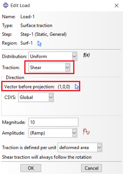
Figure 6: Edit load dialog box for Surface Traction load
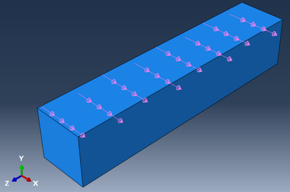
Figure 7: applied Surface Traction Load
Now, let’s make some practical examples in the real-world to understand the surface traction.
Shear Traction: In shear traction, the force acts parallel to the surface, simulating frictional forces. A good example of this is the interaction between a car’s tire and the road. As the tire moves forward, friction acts along the surface of the road, creating shear traction. This is a key aspect of how vehicles maintain grip on the road, especially during turns or braking.
General Traction: General traction allows you to specify forces acting in any direction. A practical example is wind pressure on the surface of a skyscraper. Wind doesn’t always blow head-on; it often hits at different angles. This uneven pressure creates a combination of normal and tangential forces that act across the building’s surface. With general traction, you can simulate this complex loading behavior by defining the direction of the forces.
2.1.4. Moment
Moment is a rotational force applied to create a bending or twisting effect on a structure, such as torque applied to a shaft.
To apply torque in Abaqus (Abaqus Moment Load), after selecting Moment as the load type, a point must be selected as the location of torque application, and then the magnitude for all three axes must be determined.
As you can see in Figure 8, the torque in each direction is indicated by two arrows.
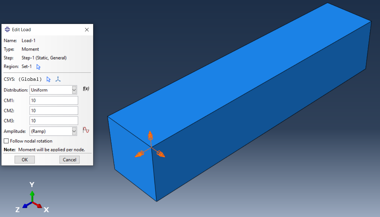
Figure 8: Torque applied to a point of the specimen
2.1.5. Abaqus Shell Edge Load
Abaqus Shell Edge Load is a load applied along the edge of shell elements, often used in thin-walled structures like plates and shells. It simulates forces along edges, such as tension along the edges of a stretched fabric. For instance, in a trampoline, the fabric is stretched tightly.
To apply this type of loading, one edge of the shell element must be selected and the magnitude must be specified. It should be noted that in this loading, the magnitude of the force is per unit length.
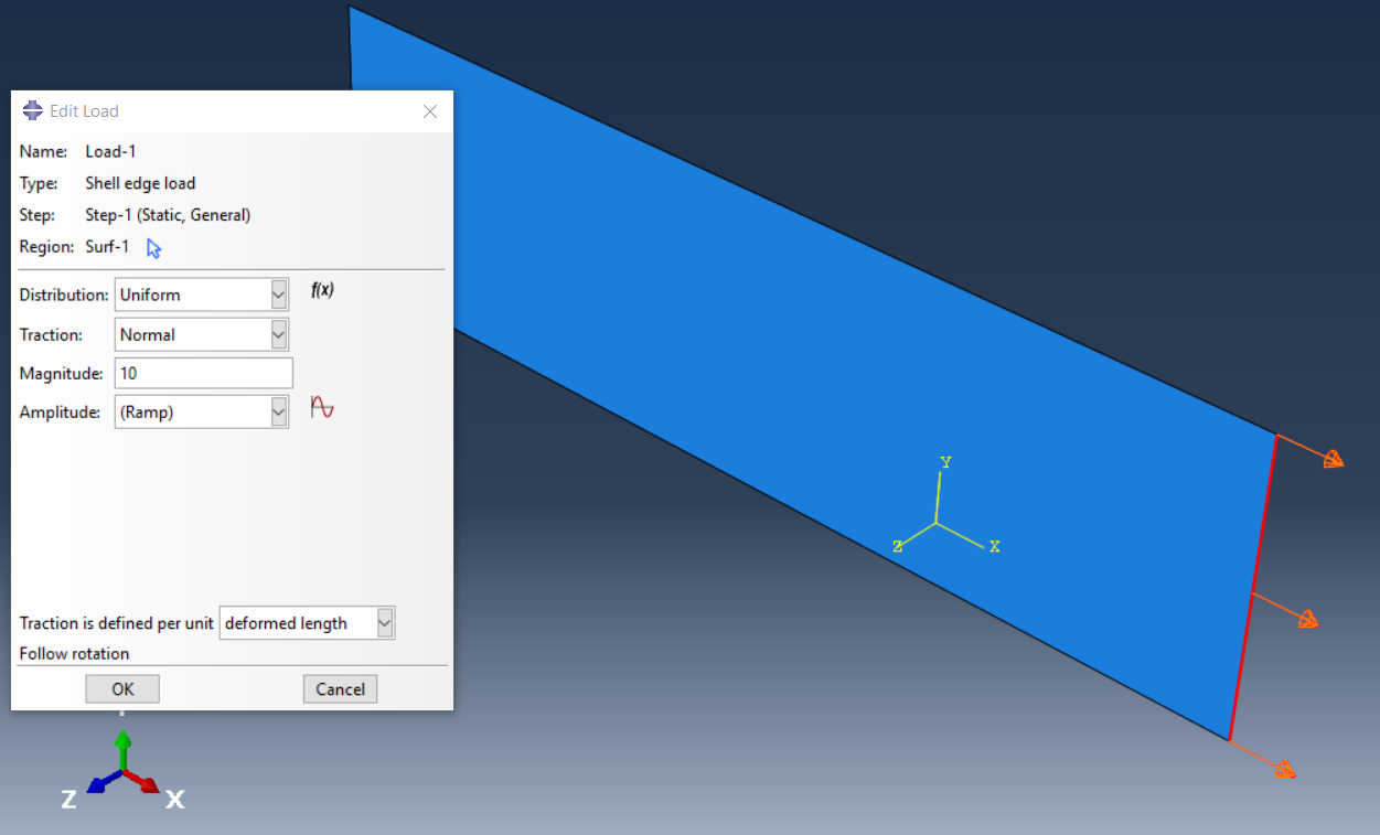
Figure 9: Shell Edge Load applied on shell element
As you can see in Figure 10, there are 5 different modes for applying this force on the edge of the element.
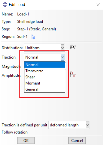
Figure 10: Traction types for Shell Edge Load
- Normal: Normal traction is applied perpendicular to the edge of the shell.
- Transverse: Transverse traction is applied in the plane of the shell, perpendicular to the edge, and Normal traction.
- Shear: Shear force applied in the plane of the shell, perpendicular to the edge.
- Moment: Bending moment applied along the edge, creating rotational effects.
- General: Allows you to define a custom direction for the force.
In the figure 11 you can see all these tractions that have been applied.
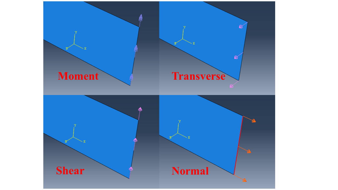
Figure 11: Traction types
Abaqus shell edge loads are essential for simulating real-world scenarios where forces act along the edges of thin-walled structures. Understanding the different types of shell edge loads can help engineers model and analyze various applications accurately. Below, we explore practical examples for each type of shell edge load.
Normal Traction
Example: Tension in a Fabric Structure
Consider a large tent made of fabric. The edges of the tent are subjected to tension as they are anchored to the ground. In Abaqus, normal traction can be applied to the edges of the tent’s shell elements to simulate this tension. This load acts perpendicular to the edge, effectively representing how the fabric stretches under wind loads or other external forces.

Figure 12: Tension in a Fabric of a tent
Transverse Traction
Example: Pressure on a Membrane
Imagine a large inflatable balloon. The surface of the balloon experiences pressure that pushes outward. In Abaqus, transverse traction can be applied to the balloon’s shell elements, simulating this internal pressure. The load acts in the plane of the shell but is perpendicular to its edge, accurately reflecting how the membrane expands under pressure.
Shear Force
Example: Shear in a Composite Panel
In aerospace applications, composite panels are often used in aircraft wings. These panels experience shear forces due to aerodynamic loads during flight. By applying shear forces in Abaqus along the edges of the shell elements representing these panels, engineers can analyze how the structure responds to these forces and ensure it meets safety standards.
We have a practical example for you to learn the shear load “Reduced Beam problem under Shear Load“.
Bending Moment
Example: Support for a Roof Structure
Consider a cantilevered roof that extends beyond its supporting walls. The roof experiences bending moments at its edges due to its weight and any additional loads like snow or equipment. In Abaqus, a bending moment can be applied along the edges of the roof’s shell elements to simulate these effects, allowing for an accurate assessment of stress and deflection.
General Traction
Example: Custom Loading on wind turbine blade
General Traction Load: General traction lets you define a custom direction for the load. Imagine a wind turbine blade. The complex aerodynamic forces acting on the blade edges are neither purely normal, transverse, nor shear. Instead, they combine different directions, making this a perfect example of general traction where forces act in various directions along the shell’s edge.
 |
⭐⭐⭐ Free Abaqus Course | ⏰10 hours Video 👩🎓+1000 Students ♾️ Lifetime Access
✅ Module by Module Training ✅ Standard/Explicit Analyses Tutorial ✅ Subroutines (UMAT) Training … ✅ Python Scripting Lesson & Examples |
2.1.6. Body Force
These loads act throughout the volume of a structure, such as gravity or centrifugal forces, and are essential for simulations involving entire bodies or large masses. These are used in cases like rotating machinery or vehicles subjected to gravitational forces.
To create this loading, a volume must be selected and the force can be adjusted in three different directions.
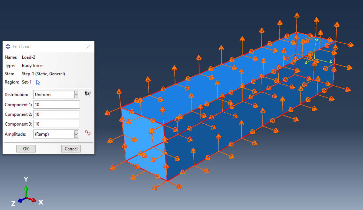
Figure 13: Body Force example
2.2. Thermal Loads
Thermal loads include temperature changes and heat flux. They are used in simulations where thermal effects, such as expansion or heat transfer, play a significant role. If you remember, the types of this category are used for solving steps related to heat transfer. In general, three types are available for this category:
- Surface Heat Flux: This load applies heat flow across the surface of your model.
- Body Heat Flux: Represents a heat source or sink distributed throughout the volume of the model.
- Concentrated Heat Flux: A localized heat load applied at a specific point or node.
These Abaqus load types are also available through the “Create Load” dialog box and the “Thermal” category.
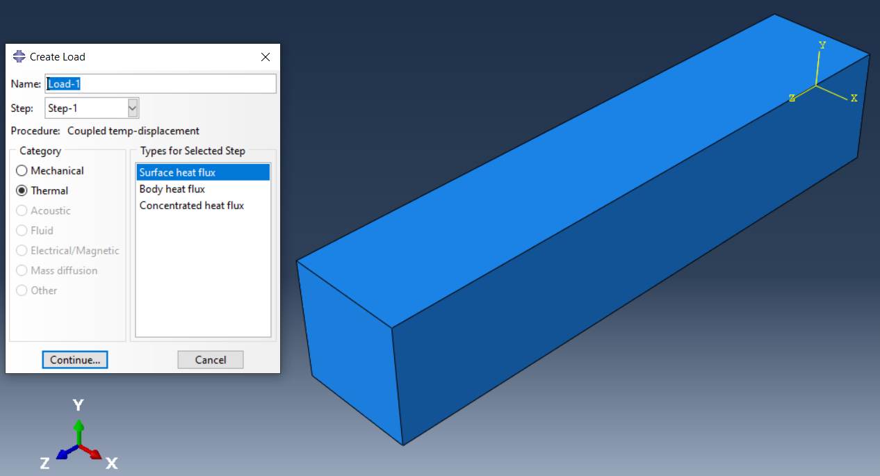
Figure 14: Thermal Category
To create a thermal load, you must first specify a surface, volume, or point according to its type, then select the magnitude corresponding to the surface or volume. For example, Figure 15 uses the surface heat flux type, and the magnitude value is expressed per surface unit.
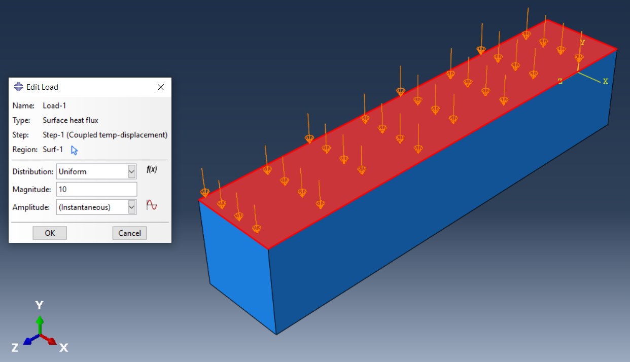
Figure 15: Creating surface heat flux load
There is a blog covers all you need to know about heat transfer and thermal analysis specially simulating it in Abaqus; the blog titled: “An overview – Heat Transfer and Thermal Stress Analysis with Abaqus“.
2.3. Acoustic Loads
These loads are used in simulations involving sound waves, particularly in studies of acoustics or vibrations in fluid-filled domains. They simulate pressure loads within an acoustic area.
For this category Inward volume acceleration loading type is available. Inward volume acceleration represents a type of distributed load applied to the nodes of acoustic elements at the boundary of an acoustic medium. It is essentially an acceleration force per unit mass that acts inward toward the medium. The load is derived from integrating pressure gradients over a surface area, resulting in a volumetric acceleration.
In acoustic analysis, distributed loads (like pressure gradients) are interpreted as forces per unit mass (acceleration). These loads can act on the boundaries of the acoustic domain. The load’s effect is modeled as the acceleration of the fluid medium at the boundary, such as when a rigid plate oscillates vertically, imposing acceleration on the acoustic fluid.
Inward Volume Acceleration is a critical load type in acoustic simulations, representing acceleration forces applied to an acoustic medium’s boundary. It is used in both frequency domain and transient dynamic analyses to simulate wave propagation and the interaction of sound with surrounding structures.
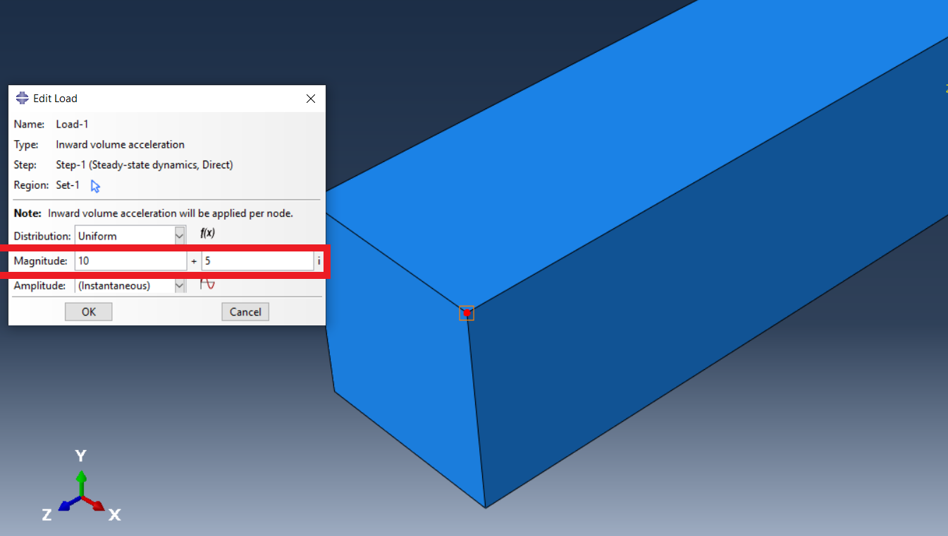
Figure 16: Applying inward volume acceleration
As you can see in figure 16 after selecting a node, to specify the magnitude of this loading, you can enter a complex number. In frequency domain (harmonic) analysis loads like Inward Volume Acceleration are oscillatory and vary with time. A complex number allows you to represent both the magnitude (real part) and phase shift (imaginary part) of the oscillating load.
2.4. Electrical and Magnetic Loads
Electrical and magnetic loads simulate electromagnetic effects in structures, such as applying electric potentials or magnetic fields. These are used in studies involving electromagnetism and its interaction with materials.
As you can see in Figure 17, this category also has three different types. Based on these types, you can determine the passing current based on the geometry. A point, surface, or volume of the sample can be selected to pass the current. Remember that the magnitude in each is based on the current passing per unit of cross-section. For example, for the type of surface current, the magnitude is expressed based on the current per unit area.
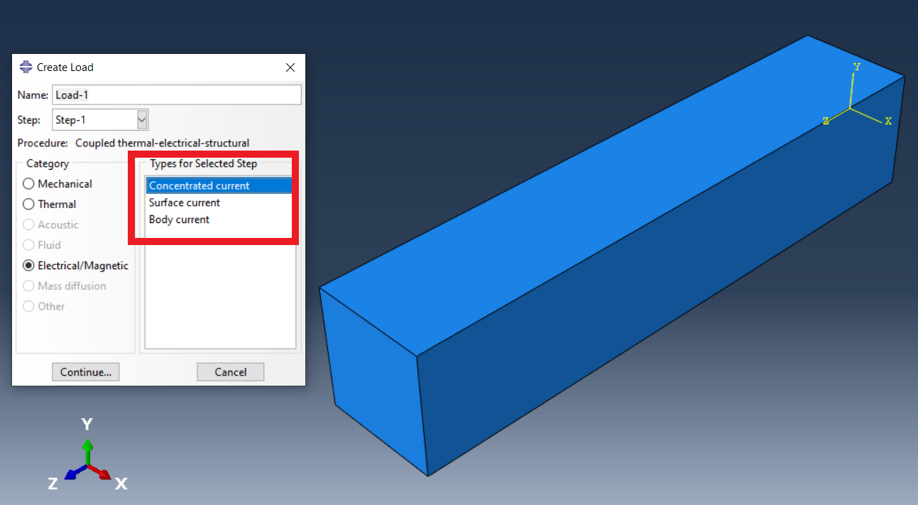
Figure 17: Electrical and magnetic Abaqus load types
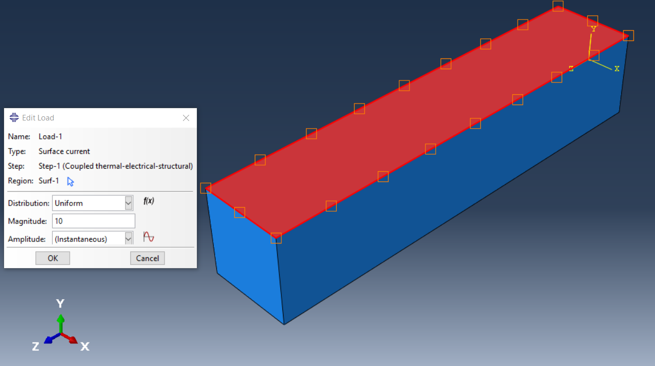
Figure 18: Surface current load type
We’ve discussed the units for some of these loads, but haven’t specified whether they’re SI units, millimeters, or something else. That’s because Abaqus doesn’t inherently include units for quantities. However, the article “Used Units in Abaqus | Abaqus Units” can help you understand the units used in the software.
2.5. Fluid Loads
Fluid loads include forces exerted by fluids on structures, such as fluid pressure on submerged surfaces or the effect of fluid flow around objects. These loads are essential in simulations involving fluid-structure interactions, such as in pipes, tanks, or hydraulic systems.
The Fluid category in Abaqus is used to apply loads related to fluid flow within porous media, particularly in geotechnical and consolidation analyses. This category allows you to simulate the behavior of fluids moving through a porous material by prescribing pore fluid flows or seepage conditions on the elements or surfaces. This is often used in geotechnical engineering to simulate phenomena like groundwater flow, drainage, or the behavior of water in soil under load.
This loading is also available with two types of surface pore fluid and concentrated pore fluid. As you may have guessed, to create this loading type, you need to select the surface and the point respectively. You can then apply these loadings by determining the magnitude. Remember The magnitude of the Surface Pore Fluid Load type in Abaqus represents the fluid velocity across the surface due to pore pressure differences.
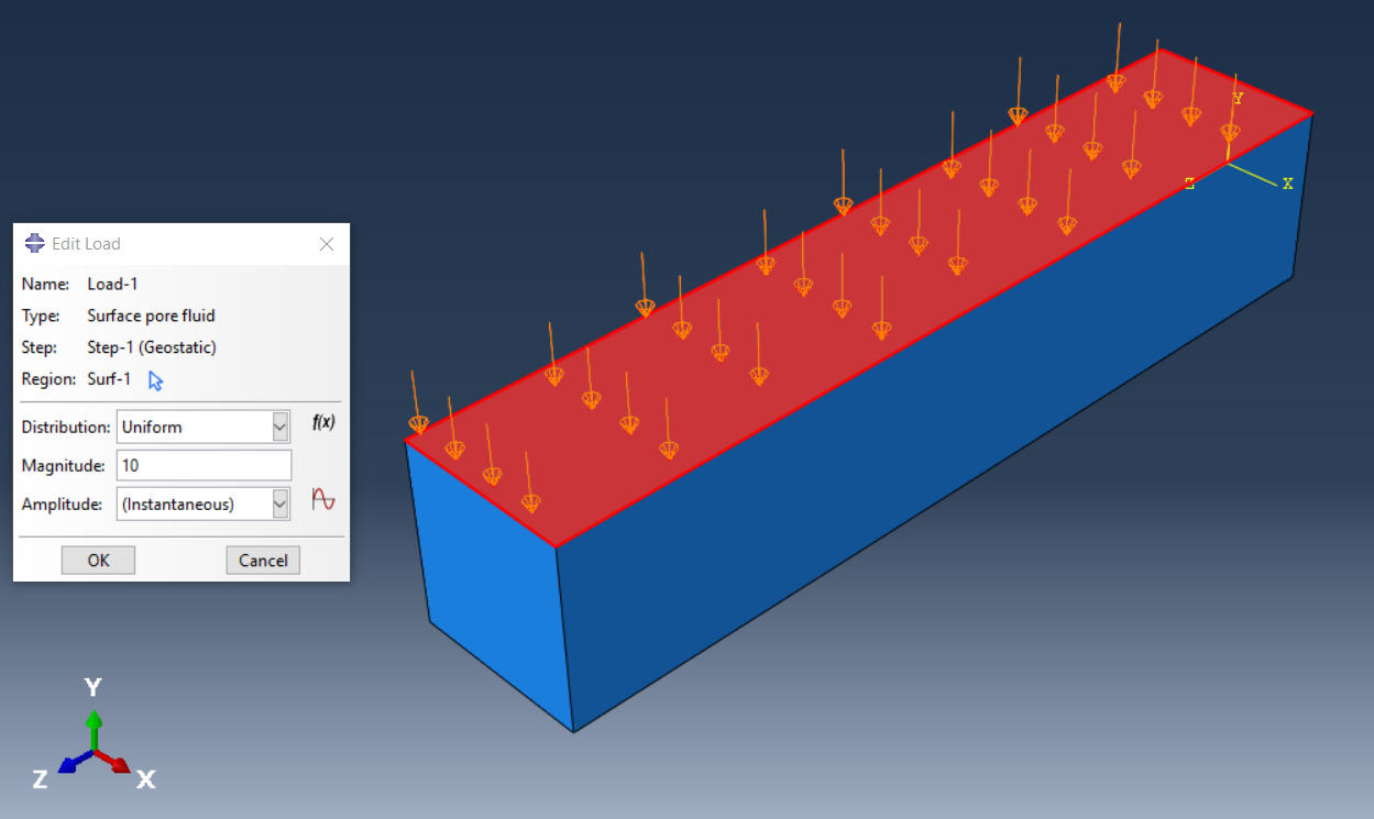
Figure 19: Surface pore fluid load type
2.6. Mass Diffusion Loads
The Mass Diffusion load category in Abaqus deals with the process of mass transfer within a material, often involving the diffusion of a substance (such as gas, liquid, or solute) through a solid medium. In these analyses, the primary objective is to model how the concentration of the diffusing material evolves over time and space within the domain.
This category includes three Abaqus load types, with the first being a concentrated concentration flux, which is a point load applied to specific nodes within the model. This flux represents the rate of mass entering or leaving the system at a particular point. The load is defined by specifying the node (or set of nodes) and the magnitude of the flux. This type of load is used when the mass flux is concentrated at discrete locations rather than distributed over a surface or volume. The surface concentration flux and the body concentration flux also act like the concentrated concentration flux, with the difference that in these two types, the material passes through the surface and the volume, respectively.
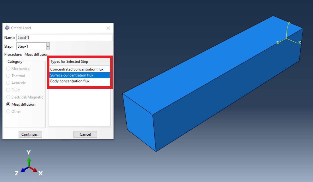
Figure 20: Mass diffusion load types
3. Abaqus load amplitude
In the previous sections, you might have noticed the option to enter an amplitude when specifying the magnitude. But what exactly is amplitude? How is it used? And how does it affect the applied magnitude? Let’s explore these questions in more detail in this section.
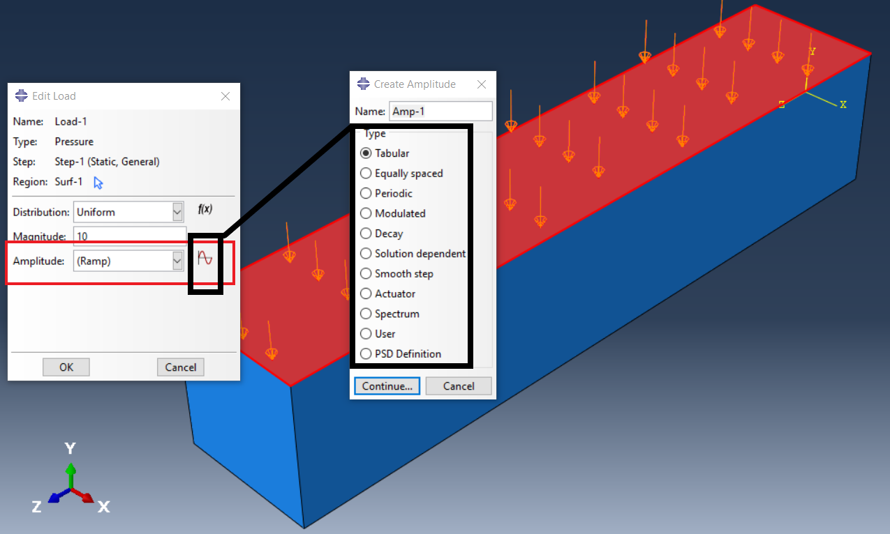
Figure 21: “Create Amplitude” dialog box
In Abaqus, load amplitude is crucial for defining how loads and boundary conditions vary over time during an analysis. Amplitudes allow you to control the magnitude of a load or boundary condition at specific points in time, which is essential for simulating real-world conditions such as varying forces, pressures, or displacements. Using load amplitudes enables the modeling of dynamic effects, ramp-up periods, and load cycles in various structural and non-structural analyses.
For example, consider a bridge structure subjected to a gradually increasing load as vehicles move across it. Instead of applying the maximum load instantaneously, which is unrealistic, a ramped amplitude can be used to simulate the gradual increase of load as vehicles move onto the bridge and then gradually decrease it as they move off. This approach gives a more accurate representation of the real-world loading scenario.
If you’re interested in learning about Abaqus Amplitude types, understanding their graphical representations, and exploring practical examples, I recommend checking out the article “Abaqus Amplitude.” This resource will also guide you through advanced topics like the “UAMP subroutine.“
4. What are DLOAD and VDLOAD subroutines?
You may have encountered loadings in your modeling that were not present in Abaqus default load types. But Abaqus has provided a solution for this problem by using DLOAD and VDLOAD subroutines. DLOAD and VDLOAD are user-defined subroutines in Abaqus that allow you to define custom loads in simulations. These subroutines are particularly useful when you need to apply complex or non-standard loads that cannot be easily represented using the standard Abaqus load types.
- DLOAD: This subroutine is used in static and quasi-static analyses to define distributed loads as a function of position, time, or other parameters.
- VDLOAD: This subroutine is similar to DLOAD but is used in dynamic analyses, where the load can vary with time and velocity.
Both subroutines give users the flexibility to implement load conditions that are not predefined in Abaqus, which can be particularly useful for advanced simulations where loading conditions are complex, variable, or dependent on multiple factors.
- How DLOAD Subroutine works: In static or quasi-static analyses, the DLOAD subroutine is called at each integration point for each element face where a load is applied. You can define the load as a function of position, time, and other variables. The subroutine then calculates the magnitude of the distributed load for each element face.
- How VDLOAD Subroutine works: In dynamic analyses, the VDLOAD subroutine works similarly to DLOAD but adds the ability to define loads that depend on the velocity of nodes or elements. This is particularly important for simulating dynamic effects such as wind loading, where the load intensity varies with speed.
 |
This training package helps Abaqus users to prepare complex DLOAD and VDLOAD subroutines. With the help of these workshops, you can get acquainted with the basic and comprehensive way of DLoad and VLoad subroutine writing and their applications. By viewing this package as an engineer, you can do basic projects with complex loads. |
5. Conclusion
This article focused on understanding the different types of loads in Abaqus and their proper application in simulations. The ability to accurately define loads is critical in achieving reliable results in finite element analysis.
Accurately applying loads in Abaqus is fundamental to preventing design failures and ensuring the safety of real-world applications. Throughout this article, we delved into various load categories, including mechanical, thermal, fluid, and mass diffusion loads. We also reviewed detailed examples of creating different types of loads for each category such as concentrated forces, pressure loads, surface traction, surface heat flux, surface current, and etc. this article showed how each type of load is created in Abaqus, what parameters for applying is needed and how it affects a model. On the other hand, the importance of amplitudes was highlighted in defining how these loads evolve over time, and different types of amplitudes including tabular, periodic, decay, and etc. were investigated. Additionally, advanced features like the DLOAD and VDLOAD subroutines were introduced, enabling users to customize loads for complex scenarios that go beyond Abaqus GUI (graphical user interface) capabilities.
In conclusion, understanding the various load types in Abaqus and applying them correctly is vital for achieving accurate simulations, ensuring realistic results, and avoiding potential design failures.
The CAE Assistant is committed to addressing all your CAE needs, and your feedback greatly assists us in achieving this goal. If you have any questions or encounter complications, please feel free to share it with us through our social media accounts including WhatsApp.
Explore our comprehensive Abaqus tutorial page, featuring free PDF guides and detailed videos for all skill levels. Discover both free and premium packages, along with essential information to master Abaqus efficiently. Start your journey with our Abaqus tutorial now!
Of course you can always learn more in detail about Abaqus in Abaqus Documentation.