
Abaqus UEL & VUEL subroutines: Intro, Variables, Abaqus UEL Example

Have you ever thought about having custom elements in Abaqus? Abaqus provides many built-in elements, but sometimes they are not enough for specialized simulations. If you need to model complex materials, unique geometries, or advanced physical behaviors, the default options may not work. This is where the Abaqus UEL (User ELement) subroutine becomes useful.
The UEL and VUEL subroutines allow users to define custom elements by programming their stiffness matrix, mass matrix, and internal forces. This flexibility makes them valuable for researchers and engineers working on innovative simulations that Abaqus elements cannot handle. It is commonly used in cases like micromechanical modeling, coupled-field problems, and experimental finite elements.
In this blog, we introduce the UEL and VUEL subroutines, explaining how they work and when to use them. We also compare UEL with UELMAT, another subroutine that includes custom material models. Additionally, we go through the key variables of UEL and VUEL and provide a step-by-step example of implementing UEL in a truss simulation. By the end, you will have a clear understanding of how to start using UEL in Abaqus.
So the UEL and VUEL subroutines are for advanced users and they hard to learn, right? But we’ve got you covered! Whether you’re just starting out, diving into advanced custom elements, or focusing specifically on VUEL, these tutorials will take you from beginner to expert. Our Beginner UEL Tutorial lays the foundation in simple terms, the Advanced UEL Guide pushes your skills further with complex implementations, and the Special VUEL Tutorial is your go-to for everything VUEL. No more confusion—just clear, step-by-step guidance. Ready to take your Abaqus skills to the next level? Click below and start learning!
|
First steps in learning UEL subroutine: UEL for Beginners |
Next step in learning UEL subroutine: UEL Advanced Level |
Final step is learning VUEL Subroutine |
1. What is the UEL Subroutine?
The UEL (User ELement) subroutine in Abaqus/Standard allows advanced users to define custom element behaviors beyond the capabilities of predefined Abaqus elements. With UEL, users can specify how an element behaves during analysis by programming its stiffness matrix, mass matrix, residual force vector, and energy contributions.
1.1. Why should we use the UEL subroutine?
When built-in Abaqus elements are Inappropriate for a specific analysis, UEL allows users to tailor element formulations to their requirements. It enables the simulation of advanced behaviours like non-standard constitutive models. Also, UEL is particularly useful in academic or industrial research where new materials or unique physical phenomena require custom modelling.
1.2. Examples of UEL subroutine applications
- Special Beam and Shell Elements: Standard beam and shell elements in Abaqus assume classical beam/shell theories. If an analysis requires higher-order beam theories or custom composite shell formulations, UEL is needed.
- Custom Geometry: If the problem requires elements with special geometry, such as an element for irregular shapes, UEL allows you to define the nodes and how they interact.
- Coupled Field Problems: Developing elements for scenarios such as thermos-mechanical or electro-mechanical couplings that cannot be handled using elements available in Abaqus
- Experimental Elements: Introducing elements for research purposes, such as a novel finite element method, that UEL allows to implement new ideas.
- Micromechanical Models: Simulating material behavior at the microscopic level, like grains in a metal, where the material’s behavior depends on the microstructure.
- Bioengineering and Soft Tissue Modelling: Soft biological tissues exhibit viscoelastic, anisotropic, and nonlinear mechanical behavior, which standard elements may not fully describe. UEL allows for custom formulations of muscle, skin, or organ tissues, improving the realism of biomedical simulations.
- Functionally Graded Material (FGM) Elements: FGMs have gradually varying material properties across their volume (or length or surface), which is difficult to model with standard elements. A UEL subroutine can define elements where stiffness, thermal expansion, and conductivity vary continuously, allowing accurate simulation.
2. Abaqus UEL tutorial: guide to writing UEL subroutine step by step
To write and implement a UEL subroutine in Abaqus, you must first become familiar with its interface, variables, and how to connect and transfer data between the software and the UEL subroutine. In this Abaqus UEL tutorial, first, the UEL interface then UEL variables will be introduced.
2.1. UEL subroutine interface
The first step in this process is to understand the UEL subroutine interface. Abaqus has defined a specific format and several variables for each subroutine, just like UEL. Users must follow this format to use subroutines. Here is the UEL subroutine interface.
New to UEL subroutines? Start with our beginner-friendly guide and learn the basics step by step! The intro of this tutorial is about “when we need it? How does the UEL subroutine work? What is the UEL subroutine interface?, etc.”
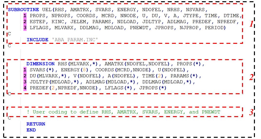
Figure 1: UEL subroutine interface
The subroutine is called at every increment of the analysis for the user-defined element type. As you can see in Figure 1, the UEL subroutine consists of three parts. The first part introduces the variables used in the subroutine. The second part specifies the dimensions of the variables, and in the third part, Abaqus provides various input variables to the UEL subroutine, and users are responsible for defining the “To be defined” such as RHS, and AMATRX variables.
2.2. What are UEL subroutine variables?
The UEL subroutine, like other subroutines has its own variables specified by Abaqus. Some of these variables are “to be defined” variables and must be defined and calculated by the user and are known as outputs and their calculation is essential. However, the rest of the variables are not essential and can only be used in the process of calculating the “to be defined” variables and help the user. These variables are “Passed in for information”. In the table below, the UEL subroutine variables are introduced, and described, and their types are also specified.
|
Variable |
Type | Description |
| RHS | To be defined |
The residual force vector for the element, representing the internal forces that contribute to the global system of equations. It must be correctly calculated because Abaqus assembles it into the force balance equation. In simple terms, this array contains the forces or fluxes for the element (these forces are used in the equations for determining the stiffness matrix). |
| AMATRX | To be defined |
Characteristic matrices such as the stiffness (Jacobian) matrix (or the inertia matrix), determine how the element resists deformation. The AMATRX must be fully defined; otherwise, Abaqus assumes a symmetric stiffness matrix. |
| SVARS | To be defined |
Solution-dependent state variables that store material history (e.g., plastic strain, damage variables, etc.). These variables are defined by the user for unforeseen applications for which no variables are defined by Abaqus and must be updated at each increment. |
| ENERGY |
To be defined (if energy tracking is needed) |
Energy contributions associated with the element. It must be updated if energy tracking is required. The 8 components ENERGY array include: (1) Kinetic energy, (2) Elastic strain energy, (3) Creep dissipation, (4) Plastic dissipation, (5) Viscous dissipation, (6) Artificial strain energy, (7) Electrostatic energy, (8) Incremental work done by external loads. If left undefined, Abaqus assumes zero energy contribution. |
| PNEWDT |
Can be updated (if time stepping control is needed) |
Ratio of suggested new time increment to the time increment currently being used. This variable can only be used when automatic time incrementation mode is enabled. This variable allows you to provide input to the automatic time incrementation algorithms and improve that. |
|
NDOFEL |
Passed in for information |
This variable specifies the number of degrees of freedom of the element. |
|
PROPS |
Passed in for information |
Real-valued properties of the element (e.g., material constants like Young’s modulus, thickness). These values are defined in the input file with UEL PROPERTY. |
| JPROPS | Passed in for information |
Number of integer properties assigned to the element. |
| COORDS | Passed in for information |
Nodal coordinates of the element at the beginning of the analysis. These remain constant throughout the simulation and are used to calculate strain-displacement relationships. |
| U | Passed in for information |
Field variables such as displacements (in structural analysis) at the element’s nodes, accumulated from the beginning of the analysis. Used for computing strains. |
|
DU, V, A |
Passed in for information |
Incremental field variable (e.g., displacement) for the current increment, nodal first derivative (velocity), and nodal second derivative (acceleration) respectively. |
In the table above, you were introduced to the most important variables of the UEL subroutine, but these were brief and short explanations. On the other hand, some other variables were not explained in this table. Therefore, you can use “Introduction to UEL Subroutine in ABAQUS” package to become fully familiar with all the variables and learn the details related to this subroutine.
3. What is the VUEL Subroutine?
The VUEL (User ELement for Explicit) subroutine is used in Abaqus/Explicit to define custom finite elements. It is the explicit dynamic version of the UEL subroutine, which is used in Abaqus/Standard. In Abaqus/Explicit, mass and forces are the primary governing factors, unlike in Abaqus/Standard, where the equilibrium equation is based on stiffness matrices. Since explicit methods do not use a global stiffness matrix, VUEL does not require stiffness matrix calculations (AMATRX), unlike UEL.
3.1. VUEL Subroutine Interface
The VUEL subroutine also has its own interface. This interface differs from the UEL subroutine due to the type of solvers used in these subroutines. Below is the VUEL subroutine interface:
Curious about VUEL? This hands-on tutorial will make writing VUEL subroutines easier than ever! The intro of this tutorial is about “when we need it? How does the VUEL subroutine work? What is the VUEL subroutine interface?, etc.” 2 Educational Workshops.
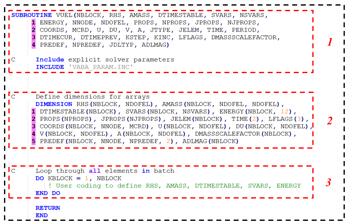
Figure 2: VUEL subroutine interface
As you can see, this subroutine, like other subroutines, consists of three parts. The first part is to define the variables of the subroutine, and the second part is to specify the dimensions of the variables, but in the third part, the user must define the necessary variables inside a DO loop.
3.2. VUEL Subroutine Variables
As with other subroutines, accurate knowledge of VUEL variables plays an important role in the correct use of this subroutine. Due to the closeness of the VUEL subroutine’s application to UEL, many of the variables of these two subroutines are exactly the same. However, due to minor differences in the subroutines, especially the solver, a number of variables are different. Below is a table of variables that are unique to the VUEL subroutine and not found in UEL. Keep in mind that VUEL doesn’t include all of the UEL variables. Both subroutines share some variables, but each also has its own distinct set.
|
Variable |
Type | Description |
| AMASS | To be defined |
The mass matrix of the element. Unlike UEL, where the stiffness matrix (AMATRX) is required, explicit analysis depends on mass. You must define this matrix to properly account for inertia effects. |
| DTIMESTABLE | To be defined |
The maximum stable time increment for each element. If this is not defined correctly, the simulation may crash. |
| DMASSSCALEFACTOR |
To be defined (if mass scaling is used) |
A mass scaling factor that increases the element’s mass to artificially increase the stable time step. This is optional but useful for speeding up simulations where very small time steps are an issue. |
| NBLOCK |
Passed in for information |
The number of elements being processed in this subroutine call. Since Abaqus/Explicit processes elements in batches, this helps improve efficiency. |
| DTIMECUR |
Passed in for information |
The current time increment in explicit analysis. This is updated every increment. It is mainly used for reference and is not modified by the user. |
|
DTIMEPREV |
Passed in for information |
The previous time increment from the last calculation. It helps track how the time step changes over the course of the analysis. |
On the other hand, some variables of these two subroutines have different names but are very similar in use. For example, we can mention the variables AMATRX and AMASS. While variable AMATRX is usually used in the UEL subroutine to calculate the stiffness matrix, in the VUEL matrix variable AMASS is the mass matrix. These two variables are different but have the same role in the subroutine solution process.
A VUEL subroutine, like UEL, is a complex subroutine. There are also other variables that are not included in Table 2, and using these variables correctly in the subroutine writing process can be challenging. However, the “Introduction to VUEL subroutine in ABAQUS” package can guide and help you in the process of writing a VUEL subroutine correctly.
4. Abaqus UEL Example
As mentioned, UEL subroutines can be used in various issues where new elements need to be defined. To learn more about UEL subroutines, let’s look at a very simple example together. However, we have an advanced example as well in this tutorial: “UEL advanced level“
Simulation of a Truss using UEL subroutine in Abaqus:
Although it is possible to simulate a 2D or 3D truss well using the default elements available in Abaqus, the reason for choosing this example is the simplicity of the education and the simulation of the truss with the UEL subroutine in Abaqus.
As you can see in the figure below, in this example, a truss with two links will be simulated. This truss will be subjected to a concentrated load of 100 Pascals from the connection of the links. You can also see in the figure the truss supports that are fixed.
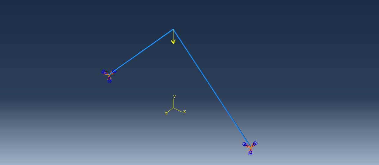
Figure 3: Truss simulation schematic
Since Abaqus does not allow users to directly access the UEL subroutine through the graphical user interface (GUI), this must be done using the .inp file. Changes made to this file to access the UEL subroutine must be made according to the instructions provided by Abaqus. These instructions are available in the Abaqus documentation.
In the figure below, you can see the changes made to the .inp file for the truss example. These changes include properties, element names, and etc.
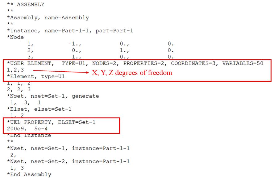
Figure 4: User element changes in .inp file
- TYPE: The first change is TYPE. This parameter is equal to the element type key used to identify this element on the ELEMENT option. The format of this type of key must be Un, where n is a positive integer less than 10000. In simple terms, TYPE is used to identify elements.
- NODES: Should be set equal to the number of nodes associated with an element of the same type. Note that for simplicity, each truss link is considered to be an element, so each element has two nodes.
- PROPERTIES: Should be equal to the number of real (floating point) property values needed as data in the user subroutine UEL to define such an element (number of PROPS).
- VARIABLES: It is equal to the number of solution-dependent state variables that must be stored within the element.
- COORDINATES: Shows the dimension. As you can see in the figure, numbers 1, 2, and 3 list the active degrees of freedom at the first node of the element. It means that the node can move through X, Y, and Z directions.
- UEL PROPERTIES: User should also add the material properties to the .inp file. As you can see, the elastic modulus is 200 GPa and the cross-sectional area of each element is 5 cm2.
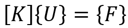
The next step in the example is to write the subroutine, but before that, it is necessary to examine the theory considered for the element’s behavior. Because in this example, the displacement of the elements is only considered, to define the behavior of the elements, we only consider the change in their length. For this, we can consider the change in the length of the elements as a spring, so the behavior of the elements follows the following relationship. This equation is written in the local system.
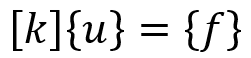
Where k is the stiffness, u is the displacement, and f is the resultant of the forces. The stiffness matrix for the symmetric problem is defined as follows:
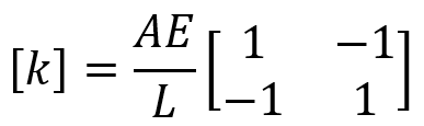
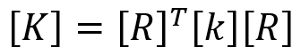
Where E is the elastic modulus, A is the cross-sectional area, and L is the length of the element. However, you should keep in mind that the UEL subroutine requires users to do calculations in the global system. Therefore, we rewrite the equation as follows:
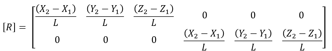
In the Global system, K is calculated by this equation:
Which R matrix is equal to:
Now we can write the UEL subroutine. The main goal in writing the UEL subroutine is to define the variables AMATRX and RHS. In the image below, you can see the process of calculating these two variables in the subroutine.
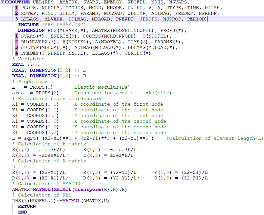
Figure 5: UEL subroutine for truss example
In this subroutine, first, the coordinates of the beginning and end of the element (the coordinates of the first and second nodes) are extracted using the COORDS variable. Then, using this data, the length of the element (L), is calculated.
In the next step, the k matrix in the local system and the R matrix were calculated using the relations described before. Then, by matrix multiplication of these two variables, the left side of the equilibrium system, or the AMATRX matrix, was calculated.
And finally, the RHS variable (right side of the equilibrium system) which is the resultant of the internal and external forces must be calculated. This variable can be calculated by multiplying the K matrix by the displacement matrix (U) in the global system. Remember that the dimension of this matrix is equal to the number of degrees of freedom of the nodes and the number of nodes.
Now by running this subroutine, you can see the results obtained. The figure below shows the displacement in the truss after applying force.
Try an advanced example this time in UEL subroutine! Ready to level up? Master advanced UEL techniques and push the limits of Abaqus!
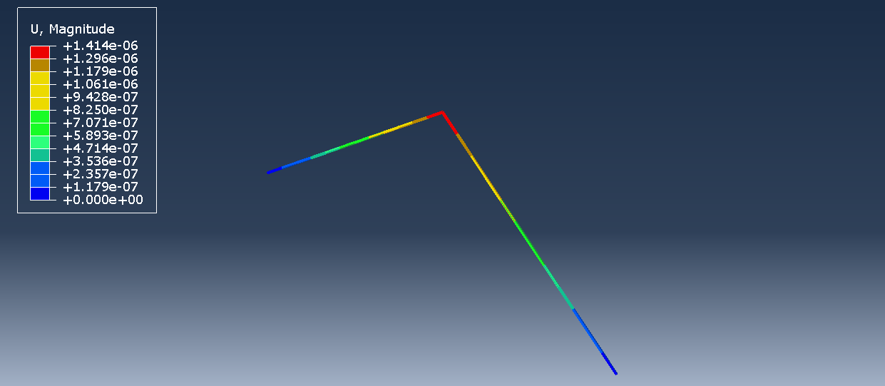
Figure 6: the result of the simulation truss using the UEL subroutine
So the UEL and VUEL subroutines are for advanced users and they hard to learn, right? But we’ve got you covered! Whether you’re just starting out, diving into advanced custom elements, or focusing specifically on VUEL, these tutorials will take you from beginner to expert. Our Beginner UEL Tutorial lays the foundation in simple terms, the Advanced UEL Guide pushes your skills further with complex implementations, and the Special VUEL Tutorial is your go-to for everything VUEL. No more confusion—just clear, step-by-step guidance. Ready to take your Abaqus skills to the next level? Click below and start learning!
|
First steps in learning UEL subroutine: UEL for Beginners |
Next step in learning UEL subroutine: UEL Advanced Level |
Final step is learning VUEL Subroutine |