
Hourglass Abaqus: What is hourglassing in Abaqus?

Hourglassing is basically a weird internal movement within an element that messes up your simulation. Finite element analysis (FEA) is a powerful tool for simulating complex physical phenomena. Abaqus utilizes a variety of elements to represent the geometry of the model. However, one common challenge encountered in Abaqus simulations is “Hourglassing” (Hourglass Abaqus). This phenomenon can significantly impact the accuracy and stability of the analysis, leading to unreliable results.
The hourglass mode is a phenomenon that occurs in some finite elements during simulations where the element’s deformation exhibits an ‘hourglass’ shape. This mode of deformation can lead to unrealistic and unstable results, as it introduces artificial energy into the system. In the worst-case scenario, the hourglass mode can cause the simulation to fail.
The hourglass effect can be a challenging obstacle in Abaqus simulations. However, by understanding its causes and implementing appropriate techniques, you can effectively mitigate it and ensure accurate and reliable results.
In this article, we will talk about this phenomenon and its origins. We also mention the control methods to prevent hourglass in simulations. Let’s Start.
1. Hourglass Abaqus: Definition and Consequences
The hourglass effect is a dreaded phenomenon in finite element analysis (FEA) that can plague your Abaqus simulations, leading to inaccurate results and wasted computational resources. Hourglassing occurs when an element distorts in a non-physical manner, resembling an hourglass shape.
Imagine a perfectly square mesh element, subjected to forces. In an ideal scenario, the element deforms uniformly, maintaining its square shape. However, when elements lack sufficient stiffness in certain directions, they can deform into an hourglass shape, resembling an hourglass with a narrow waist (Figure 1). This ‘hourglassing’ mode is a zero-energy deformation mode, meaning the element deforms without any change in strain energy.

Figure 1: Elements distort to an hourglass shape in “Hourglassing” phenomenon
1.1. Consequences of Hourglassing
Hourglassing can have several negative consequences:
- Inaccurate stress and strain results
The distorted elements experience unrealistic stresses and strains, leading to inaccurate predictions of the material behavior.
- Unstable simulations
Hourglassing can destabilize the analysis, leading to divergence or termination of the simulation. These zero-energy modes can cause oscillations and instability, rendering your solution non-convergent.
- Erratic results
The presence of hourglassing can introduce noise and erratic behavior into the simulation results. Abaqus spends time and effort solving for these unreal deformations, slowing down your analysis.
Now the question is “What are the causes of the Hourglass Effect?”.
| If you need deep training, our Abaqus Course offerings have you covered. Visit our Abaqus course today to find the perfect course for your needs and take your Abaqus knowledge to the next level! |
1.2. Causes of the Hourglass Effect
Hourglassing can occur due to:
- Low-order elements
Linear elements with fewer integration points (Reduced integration) can be prone to hourglassing, as they lack the stiffness to resist distortion.
- Insufficient constraints
If the model lacks sufficient boundary conditions or constraints, the elements can easily deform in unrealistic ways.
- Large element distortions
When elements undergo significant deformation, they can lose their ability to resist shear stresses, leading to hourglassing.
The first term which is mentioned as ‘Reduced integration’ is of great importance in introducing hourglass to the model. Let’s see what reduced integration means?
2. Integration in Finite Element Methods
In FEM, the domain of interest is discretized into a set of finite elements, and the unknown function is approximated within each element using interpolation functions. Once the discrete system of algebraic equations is obtained, the integration of these equations is necessary to compute various quantities of interest, such as the internal forces, displacements, temperatures, or velocities.
Because of the complexity that exists in the models, the integration in FEM is almost performed numerically. Numerical integration is typically performed using Gaussian quadrature rules, which are based on Gaussian weights and points. The number of Gaussian points and weights depends on the dimensionality of the element and the desired degree of accuracy.
For example, a one-dimensional element with linear interpolation functions requires two Gaussian points. In general, increasing the number of Gaussian points and weights improves the accuracy of the integration, but at the cost of increased computational effort.
Based on the number of integration points considered for an element, we have two kinds of integration in FEM:
- Full integration
- Reduced Integration
Let’s see what are these two different kinds of integration.
2.1. Full integration
The expression “full integration” refers to the number of Gauss points required to integrate the polynomial terms in an element’s stiffness matrix exactly when the element has a regular shape. For hexahedral and quadrilateral elements, a “regular shape” means that the edges are straight and meet at right angles and that any edge nodes are at the midpoint of the edge.
Fully integrated, linear elements use two integration points in each direction. Thus, the three-dimensional element C3D8 uses a 2 × 2 × 2 array of integration points in the element. Fully integrated, quadratic elements use three integration points in each direction. The locations of the integration points in fully integrated, two-dimensional, quadrilateral elements are shown in figure 2.
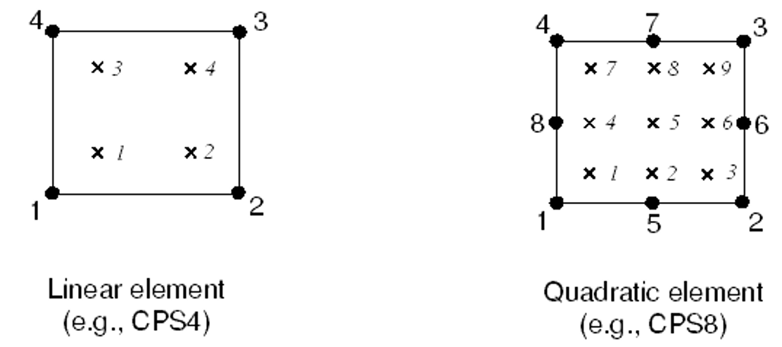
Figure 2: Integration points in fully integrated, two-dimensional, quadrilateral elements
To investigate the effect of the order of the element and integration type on FEM results, an example will be demonstrated here. This is a classic test used to assess the behavior of a given finite element. Consider a beam as shown in figure 3.
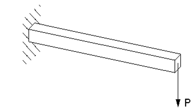
Figure 3: Cantilever beam under a point load P at its free end
The beam is 150 mm long, 2.5 mm wide, and 5 mm deep; built-in at one end; and carrying a tip load of 5 N at the free end. The material has a Young’s modulus, E, of 70 GPa and a Poisson’s ratio of 0.0. Using beam theory, for ![]() the tip deflection is 3.09 mm.
the tip deflection is 3.09 mm.
Several different meshes were used in Abaqus simulations of the cantilever beam problem, as shown in figure 4. The simulations use either linear or quadratic, fully integrated elements and illustrate the effects of both the order of the element (first versus second) and the mesh density on the accuracy of the results.
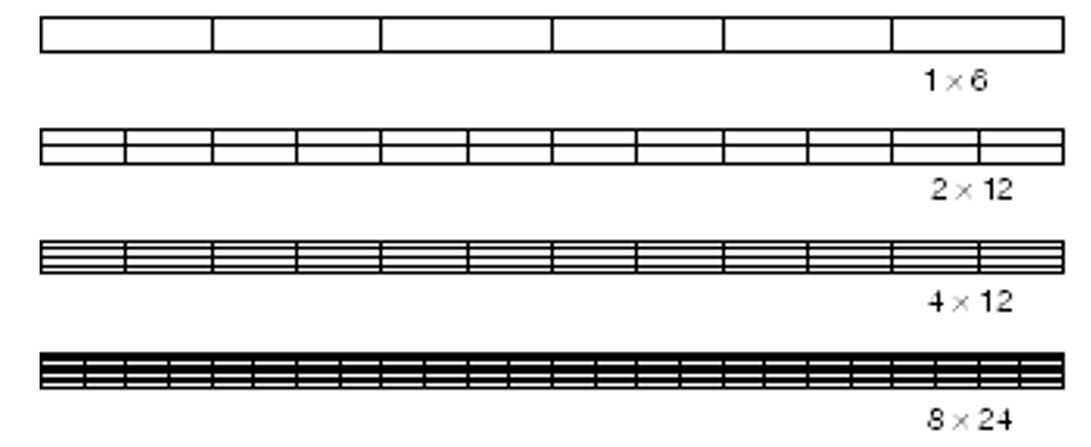
Figure 4: Meshes used for the cantilever beam simulations
The ratios of the tip displacements for the various simulations to the beam-theory value of 3.09 mm are shown in table 1.
Table 1: Normalized beam deflections with integrated elements
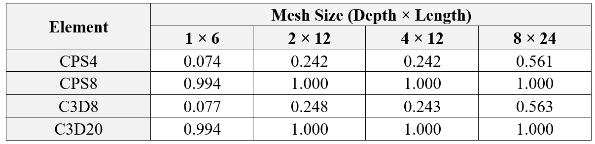
The linear elements CPS4 and C3D8 underpredict the deflection so badly that the results are unusable. The results are the least accurate with coarse meshes, but even a fine mesh (8 × 24) still predicts a tip displacement that is only 56% of the theoretical value. Notice that for the linear, fully integrated elements it makes no difference how many elements there are through the thickness of the beam. This is caused by shear locking, which is a problem with all fully integrated, first-order, solid elements.
2.1.1. Shear Locking Abaqus
As we have seen, shear locking causes the elements to be too stiff in bending. It is explained as follows.
Consider a small piece of material in a structure subject to pure bending. The material will distort as shown in figure 5. Lines initially parallel to the horizontal axis take on constant curvature, and lines through the thickness remain straight. The angle between the horizontal and vertical lines remains at 90°.
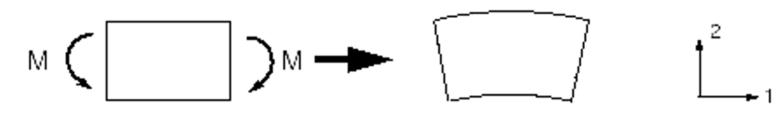
Figure 5: Deformation of material subjected to bending moment M
The edges of a linear element are unable to curve; therefore, if the small piece of material is modeled using a single element, its deformed shape is like that shown in figure 6.
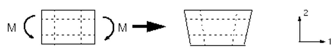
Figure 6: Deformation of a fully integrated, linear element subjected to bending moment M
For visualization, dotted lines that pass through the integration points are plotted. It is apparent that the upper line has increased in length, indicating that the direct stress in the 1-direction, ![]() , is tensile. Similarly, the length of the lower dotted line has decreased, indicating that
, is tensile. Similarly, the length of the lower dotted line has decreased, indicating that ![]() is compressive. The length of the vertical dotted lines has not changed (assuming that displacements are small); therefore,
is compressive. The length of the vertical dotted lines has not changed (assuming that displacements are small); therefore, ![]() at all integration points is zero. All this is consistent with the expected state of stress of a small piece of material subjected to pure bending.
at all integration points is zero. All this is consistent with the expected state of stress of a small piece of material subjected to pure bending.
However, at each integration point the angle between the vertical and horizontal lines, which was initially 90°, has changed. This indicates that the shear stress, ![]() , at these points is nonzero. This is incorrect: the shear stress in a piece of material under pure bending is zero.
, at these points is nonzero. This is incorrect: the shear stress in a piece of material under pure bending is zero.
This spurious shear stress arises because the edges of the element are unable to curve. Its presence means that strain energy is creating shearing deformation rather than the intended bending deformation, so the overall deflections are less: the element is too stiff.
Shear locking only affects the performance of fully integrated, linear elements subjected to bending loads. These elements function perfectly well under direct or shear loads. Shear locking is not a problem for quadratic elements since their edges are able to curve as in figure 7.
The predicted tip displacements for the quadratic elements shown in table 1 are close to the theoretical value. However, quadratic elements will also exhibit some locking if they are distorted or if the bending stress has a gradient, both of which can occur in practical problems.
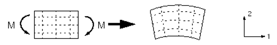
Figure 7: Deformation of a fully integrated, quadratic element subjected to bending moment M
Fully integrated, linear elements should be used only when you are fairly certain that the loads will produce minimal bending in your model. Use a different element type if you have doubts about the type of deformation the loading will create.
Fully integrated, quadratic elements can also lock under complex states of stress; thus, you should check the results carefully if they are used exclusively in your model. However, they are very useful for modeling areas where there are local stress concentrations.
 |
⭐⭐⭐Free Abaqus Course | ⏰10 hours Video 👩🎓+1000 Students ♾️ Lifetime Access
✅ Module by Module Training ✅ Standard/Explicit Analyses Tutorial ✅ Subroutines (UMAT) Training … ✅ Python Scripting Lesson & Examples |
2.2. Reduced Integration
Only quadrilateral and hexahedral elements can use a reduced-integration scheme; all wedge, tetrahedral, and triangular solid elements use full integration, although they can be used in the same mesh with reduced-integration hexahedral or quadrilateral elements.
Reduced-integration elements use one fewer integration points in each direction than the fully integrated elements. Reduced-integration, linear elements have just a single integration point located at the element’s centroid (Actually, these first-order elements in Abaqus use the more accurate “uniform strain” formulation, where average values of the strain components are computed for the element; Just for knowledge!). The locations of the integration points for reduced-integration, quadrilateral elements are shown in figure 8.
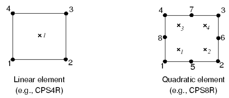
Figure 8: Integration points in two-dimensional elements with reduced integration
Abaqus simulations of the cantilever beam problem were performed using the reduced-integration versions of the same four elements utilized previously and using the four finite element meshes shown in figure 4. The results from these simulations are presented in table 2.
Table 2: Normalized beam deflections with reduced-integration elements
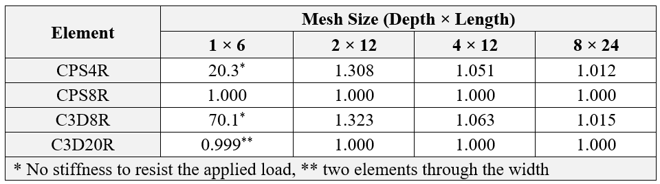
Linear reduced-integration elements tend to be too flexible because they suffer from their own numerical problem which is discussed earlier in this article: Hourglassing.
2.2.1. Hourglassing Abaqus
Again, consider a single reduced-integration element modeling a small piece of material subjected to pure bending as shown in figure 9.
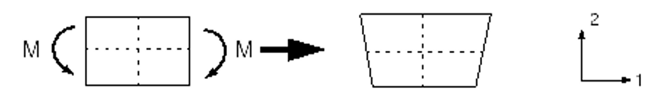
Figure 9: Deformation of a linear element with reduced integration subjected to bending moment M
Neither of the dotted visualization lines has changed in length, and the angle between them is also unchanged, which means that all components of stress at the element’s single integration point are zero.
This bending mode of deformation is thus a zero-energy mode because no strain energy is generated by this element distortion. The element is unable to resist this type of deformation since it has no stiffness in this mode. In coarse meshes this zero-energy mode can propagate through the mesh, producing meaningless results.
In Abaqus, a small amount of artificial “hourglass stiffness” is introduced in reduced-integration elements to limit the propagation of hourglass modes. This stiffness is more effective at limiting the hourglass modes when more elements are used in the model, which means that linear reduced-integration elements can give acceptable results as long as a reasonably fine mesh is used.
The errors seen with the finer meshes of linear, reduced-integration elements (Table 2) are within an acceptable range for many applications. The results suggest that at least four elements should be used through the thickness when modeling any structures carrying bending loads with this type of element. When a single linear, reduced-integration element is used through the thickness of the beam, all the integration points lie on the neutral axis and the model is unable to resist bending loads. (These cases are marked with a (*) in table 2).
Linear, reduced-integration elements are very tolerant of distortion; therefore, use a fine mesh of these elements in any simulation where the distortion levels may be very high.
Quadratic, reduced-integration elements also have hourglass modes. However, the modes are almost impossible to propagate in a normal mesh and are rarely a problem if the mesh is sufficiently fine.
The 1 × 6 mesh of C3D20R elements fails to converge because of hourglassing unless two elements are used through the width, but the more refined meshes do not fail even when only one element is used through the width.
Quadratic, reduced-integration elements are not susceptible to locking, even when subjected to complicated states of stress. Therefore, these elements are generally the best choice for most general stress/displacement simulations, except in large-displacement simulations involving very large strains and in some types of contact analyses.
Now, if you want to know more about Abaqus element types or Abaqus elements, read this article:
Introduction to Abaqus element types
Or want to know about specific types of elements read this:
3. How to control the hourglass?
Abaqus provides several mechanisms to address hourglassing:
- Element type selection
Using higher-order elements, such as quadratic or cubic elements, offers greater stiffness and reduces the likelihood of hourglassing.
- Hourglass control
Abaqus offers various hourglass control techniques, such as artificial stiffness, and viscous damping. These methods introduce artificial stiffness to the elements, preventing unrealistic distortions.
- Mesh refinement
Using a finer Abaqus mesh can reduce element distortion and mitigate hourglassing. However, this can significantly increase the computational cost.
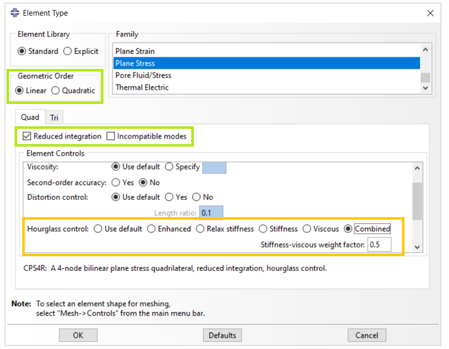
Figure 10: Abaqus hourglass control options
Now it is time to summarize what we have learned in this article.
4. Summary
We started our discussion with Abaqus’ hourglass definition and talked about the issues it will make in our analyses. For a better sight of this problem, we delved into different integration types including: Full and Reduced integration.
We demonstrated these integration types using a simple example and, in this example, we investigated the effect of the order of the element and integration type on FEM results. During this discussion, two phenomena were mentioned including Shear locking and Hourglassing.
The problems in which you may encounter these phenomena and also the available methods to solve each of these problems are introduced.
But remember, you can always find more info in Abaqus documentation.
In the end, we appreciate for reading this article. Don’t forget to leave us your comments about this article to improve our content quality. Wish you the Best.
Explore our comprehensive Abaqus tutorial page, featuring free PDF guides and detailed videos for all skill levels. Discover both free and premium packages, along with essential information to master Abaqus efficiently. Start your journey with our Abaqus tutorial now!
The CAE Assistant is committed to addressing all your CAE needs, and your feedback greatly assists us in achieving this goal. If you have any questions or encounter complications, please feel free to share it with us through our social media accounts including WhatsApp.