
Automatic Stabilization Abaqus of Unstable Problems | dissipated energy fraction, Damping factor

Have you ever set up an Abaqus simulation, hit run, and watched it crash almost instantly? Maybe the time step dropped to something microscopic. Maybe you got a cryptic error message. Or worse — maybe it just froze. If that sounds familiar, you’re not alone.
One of the most common reasons for simulation failure in Abaqus is instability. And one of the most commonly suggested fixes? Automatic stabilization in Abaqus.
But what exactly is it? How does it work? And more importantly — when should you use it, and when should you be careful?
In this guide, we’ll break down automatic stabilization Abaqus in simple terms. We’ll explain what it is, when it helps, and how to use it without risking bad results. Whether you’re new to nonlinear simulations or just tired of chasing down convergence errors, this guide is for you.
Let’s start with the basics.
Quick Reference Table
| What | Key Points |
|---|---|
| What it does | Adds artificial damping to help solve unstable problems |
| When to use | Local instability, snap-through, soft contact, debugging |
| Where to set it | Step module → Basic tab → Automatic stabilization options |
| How to set it | Choose constant damping, energy fraction, or reuse from previous step |
| Preferred method | Energy fraction with adaptive stabilization enabled |
| Validation rule | Keep ALLSD < 5–10% of ALLSE |
| Best practice | Rerun without stabilization to confirm accuracy |
| What to avoid | Overuse, ignoring energy outputs, leaving it on in final validated results |
1. What is Automatic Stabilization Abaqus?
Automatic stabilization Abaqus is a powerful tool for handling convergence issues in nonlinear static simulations. It works by adding artificial damping — like digital shock absorbers — to help the solver move through unstable parts of the model.
This feature is especially helpful when instabilities are localized. For example, if a thin shell buckles in a small area or a soft material zone starts to collapse, automatic stabilization Abaqus helps the solver avoid getting stuck. It adds just enough damping to continue solving without drastically changing the global behavior of the structure.
A good example is contact. Early in a contact simulation, small gaps or surface overlaps can cause instability. Sudden friction changes or parts not engaging properly might throw off the solver. In those cases, automatic stabilization can smooth things out. It helps form contact correctly and keeps the simulation moving.
It’s also useful in cases of rigid body motion, like when parts haven’t yet fully touched or locked in place. Or in post-buckling behavior, where stiffness changes rapidly and the solution can easily jump off course.
But — and this is important — automatic stabilization isn’t magic. If used blindly, it can hide deeper problems in the model. It adds artificial energy, so it’s crucial to monitor that energy and make sure it doesn’t interfere with real physical behavior.
There are several methods to implement automatic stabilization Abaqus:
-
Constant Damping Factor: Applies a fixed amount of damping throughout the simulation step. This method is straightforward but may not adapt well to changing conditions within the simulation.
-
Damping Based on Dissipated Energy Fraction: Calculates the damping factor based on a specified fraction of the strain energy, allowing for a more tailored approach that considers the energy dynamics of the model.
-
Adaptive Automatic Stabilization: Adjusts the damping factor dynamically during the simulation, increasing or decreasing it based on the convergence behavior. This method offers flexibility and is particularly useful for complex models with varying stability conditions.
Even though automatic stabilization can save your simulation, it’s not without risk. The added damping introduces artificial energy — and too much of it can make your results unrealistic.
That’s why it’s critical to track two energy outputs:
-
ALLSE: the total strain energy (real physical energy)
-
ALLSD: the stabilization energy (artificial energy added)
A common rule of thumb is to keep ALLSD less than 5–10% of ALLSE. If ALLSD is too high, it means the solver is relying too much on damping — and you may need to revisit your model.
In short: automatic stabilization Abaqus is a helpful tool for getting through tough spots in nonlinear simulations — especially where localized instability, contact issues, or sudden stiffness changes occur. But use it with care. Think of it as a temporary helper, not a permanent fix.
2. Why Do Simulations Become Unstable in the First Place?
Before using automatic stabilization Abaqus, it’s important to understand why simulations become unstable at all. In nonlinear FEA, convergence problems often come from three sources:
-
Geometric changes
-
Material behavior
-
Contact interactions
Let’s break each one down.
2.1. Geometric Instabilities
Sometimes, the geometry of your model is the source of trouble. As the structure deforms, its stiffness can change a lot — especially when:
-
Large displacements or rotations happen
When parts bend, twist, or stretch far from their original shape, the stiffness matrix becomes nonlinear. This makes it harder for the solver to find a solution. -
Buckling occurs
Think of a thin column under compression. It might suddenly snap sideways — that’s buckling. This sudden loss of stiffness can confuse the solver and lead to non-convergence. -
Imperfections in geometry
Even tiny flaws in the shape of a slender part can lead to big instability under load.
These are exactly the kinds of situations where automatic stabilization Abaqus can help — by smoothing out those stiffness changes just enough to keep the analysis going.
2.2. Material Instabilities
Materials can also misbehave in ways that cause convergence issues:
-
Plastic deformation
When a material yields and flows plastically, its stiffness drops. If it goes beyond your defined material data, the model may struggle to continue. -
Material softening
Some materials (like damaged concrete or ductile metals) soften as they deform. That can lead to zones where the stiffness is almost zero or even negative — which the solver doesn’t like. -
Hyperelastic materials
Rubbers and foams, which stretch a lot, can be tricky. If the model isn’t set up correctly, they can cause instability, especially under large strains.
2.3. Contact Instabilities
Contact is one of the most common causes of instability in Abaqus — and one of the trickiest to fix.
-
Initial gaps or overclosures
If surfaces start too far apart — or too close — the solver might apply unrealistic forces to force contact, leading to instability. -
Friction problems
Oversimplified friction models can make parts stick when they should slide, or slide too easily when they should grip. Both can throw off the solution. -
Changing contact status
As contact turns on or off during the simulation, stiffness changes suddenly. This can make the solver bounce around or fail to converge.
In all of these cases, automatic stabilization Abaqus can help manage the sudden shifts in contact behavior by adding controlled damping — but again, only if used carefully.
2.4. How Do You Know a Simulation Is Unstable? | Symptoms of instability
Sometimes the solver doesn’t crash — it just struggles. Here are a few signs your model might be unstable:
-
Tiny time increments
If Abaqus keeps cutting the time step smaller and smaller, it usually means it’s having trouble solving the system. -
Solver warnings
Messages like “too many attempts made for this increment” or “time increment required is less than the minimum” are red flags. -
Sudden divergence
You may see values jump wildly from one increment to the next, especially in displacements or contact pressures. -
Non-convergence after several iterations
When the solver tries repeatedly and fails to meet convergence tolerances, that’s often a symptom of deeper instability.
When you see these symptoms, it’s a signal to stop and check your model. Sometimes the fix is to improve mesh quality, adjust boundary conditions, or rethink the contact setup. Other times, automatic stabilization Abaqus might be the right tool — especially when the issue is local and not due to a bigger modeling problem.
3. When Should You Use Automatic Stabilization in Abaqus?
So now you know what causes instability and how automatic stabilization Abaqus works. But when should you actually use it?
Let’s look at the right situations — and the wrong ones.
![]() Good Use Cases
Good Use Cases
1. While debugging a model
Early in the modeling process, things don’t always work smoothly. Contact might be misaligned, boundary conditions may be too loose, or your mesh might be too coarse.
Automatic stabilization Abaqus can help get past these hiccups, so you can focus on fixing the real issues without crashing at every run.
2. Contact problems (especially soft contacts)
When simulating contact between soft parts — like rubber seals or foam padding — initial penetrations or gaps often lead to failure.
Damping helps settle these contacts gently, especially when large deformations or small surface mismatches are involved.
3. Snap-through or post-buckling problems
If your model has snap-through geometries (like domes that suddenly invert) or post-buckling behavior, the stiffness can shift dramatically.
Automatic stabilization Abaqus keeps the solver on track through those sudden changes.
4. Softening materials and damage models
Materials that lose stiffness as they deform (like concrete under crushing or ductile metals near failure) often lead to unstable zones.
In these localized areas, a bit of damping helps keep things stable without affecting global behavior much.
![]() Risks and Limitations
Risks and Limitations
Even though it helps with stability, automatic stabilization Abaqus is not without side effects.
1. Artificial energy can affect your results
Stabilization adds numerical energy (ALLSD) to the system. If this becomes too large compared to the strain energy (ALLSE), your results can become physically inaccurate.
Always track these energies and keep artificial energy below 5–10% of strain energy.
2. It can give a false sense of security
Just because a simulation converged doesn’t mean it’s correct. Overusing stabilization might hide real modeling problems — like bad contact definitions or unrealistic boundary conditions.
3. Not all instabilities should be “patched”
If the instability is global — like a model falling over due to missing constraints — stabilization won’t fix the core issue. It might just delay the error or mask it completely.
Pro Tip
Use automatic stabilization Abaqus for numerical stability, not for physical accuracy.
Don’t rely on it to fix poor modeling. Always monitor the artificial energy (ALLSD) and make sure it’s well below the real energy (ALLSE).
4. How to Use Automatic Stabilization in Abaqus?
Using automatic stabilization Abaqus isn’t just about turning it on — it’s about knowing which method to choose and how to keep your results accurate. let’s see how we can do it.
First, we need to know where to activate this setting in Abaqus CAE:
- Open your model in Abaqus/CAE.
- Go to the Step module.
- Create or edit a step (usually a static, general, or coupled temp-displacement type).
- In the Basic tab, find the section called “Automatic stabilization.”
You’ll now see three setup options:
- Specify damping factor
- Specify dissipated energy fraction
- Use damping factors from previous step
You’ll also have the option to toggle adaptive stabilization and define a maximum allowed energy ratio (we’ll explain these below).
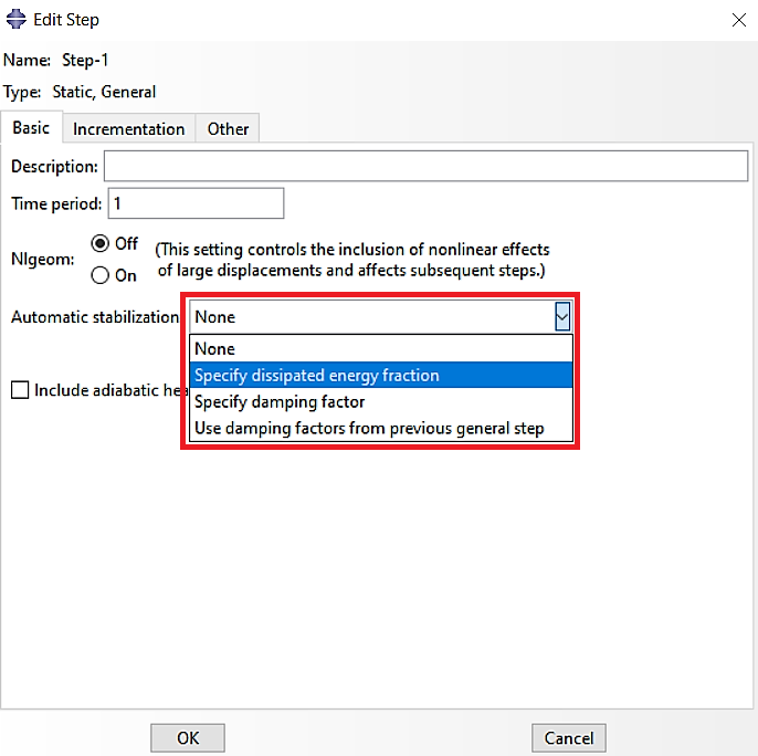 Figure 1 three different methods for Automatic stabilization
As you can see, there are three methods for automatic stabilization Abaqus which we are going to explain one by one.
4.1. Option 1: Specify damping factor (Constant)
This method applies a constant damping factor for the entire step. It introduces viscous forces of the form ![]() into the global equilibrium equations, where
into the global equilibrium equations, where ![]() is an artificial mass matrix calculated with unity density, c is a damping factor, and
is an artificial mass matrix calculated with unity density, c is a damping factor, and ![]() is the vector of nodal velocities with
is the vector of nodal velocities with ![]() being the time increment.
being the time increment.
This method is easy to apply and works well for small or simple models. However, it doesn’t adapt mid-step and needs trial-and-error to avoid over- or under-damping. bottom line, Use when you want control and are running multiple tests to find the right damping value.
4.2. Option 2: Specify Dissipated Energy Fraction (Default & Recommended)
This is the default and recommended method. You provide a small energy fraction (e.g., 2.0 × 10⁻⁴), and Abaqus calculates a damping factor so that the artificial energy (ALLSD) stays below that portion of the strain energy (ALLSE).
- This method calculates the damping factor based on the energy dissipated during the first increment of a step.
- Assumes the problem starts stable and applies damping if instabilities arise.
- The default dissipated energy fraction is 2.0 × 10⁻⁴, but this can be customized.
- If the first increment is unstable, damping is applied from the start to stabilize the solution.
Best part? This activates the adaptive stabilization scheme automatically, unless you turn it off.
This method adjusts to local changes during the step, safer and more accurate for complex or unstable models, and no guesswork on damping factor. Bottom line, Use when you want Abaqus to do the hard work and still keep artificial energy in check.
4.3. Option 3: Use Damping from the Previous Step
In long or multi-step analyses, you can choose to propagate the damping factor from a previous general step.
When to use:
-
You’ve already tuned damping in a previous step
-
You want to maintain continuity in damping behavior
-
The previous step had local instability and this one continues from it
Tip: Only use this if you’re confident the previous damping worked well.
4.4. What About Adaptive Stabilization?
Adaptive stabilization adjusts the damping factor during the step, based on:
-
Convergence history (e.g., failed iterations, cutbacks)
-
Ratio of stabilization energy (ALLSD) to strain energy (ALLSE or ALLIE)
You can toggle this feature on/off and even set a maximum allowed energy ratio. The default is 0.05 (5%) — suitable for most simulations. This is important because if damping gets too high, results can become inaccurate and if it is too low, instability can return.
Bottom line, Let Abaqus adapt — but keep an eye on the energy ratio!
4.5. Some tips
- Monitor artificial energy (ALLSD) and compare it to ALLSE or ALLIE
- Keep ALLSD below 5–10% to avoid polluting results
- Check .msg file after the first increment to see what damping factor Abaqus used
- If convergence still fails, try increasing the damping slightly — but don’t go overboard
- When done, run a follow-up step without stabilization to confirm accuracy
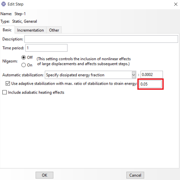 Figure 2: specify the maximum difference between ALLSD and ALLIE
When in doubt, use dissipated energy fraction with adaptive stabilization on. Don’t set damping too high — it can smooth out the wrong things and hide real problems.
5. How to Validate Your Results When Using Automatic Stabilization in Abaqus
Turning on automatic stabilization Abaqus might help your simulation run — but how do you know the results are still accurate? Here’s how to check.
Step 1: Compare Energy Outputs (ALLSE vs. ALLSD)
Abaqus provides key energy output variables:
-
ALLSE – Total strain energy (real physical energy)
-
ALLSD – Artificial energy from stabilization (viscous damping)
After your run completes:
-
Open the Visualization module in Abaqus/CAE.
-
Plot ALLSD and ALLSE vs. time or increments.
-
Check their ratio.
Rule of thumb: ALLSD should be less than 5–10% of ALLSE. If ALLSD is too high, results may be distorted. A small amount of stabilization energy is acceptable — it just keeps the system steady. Too much means your simulation may be running on numerical tricks, not physical behavior.
Step 2: Run a Comparison Without Stabilization
If your stabilized model gives good results, try this: Duplicate the step, Turn off automatic stabilization, then Run it again.
If the new run Converges easily, your model is solid; Fails completely, you likely have real instability, and if Gives different results stabilization was impacting accuracy. This test helps you see if the damping was just a nudge or a crutch.
Step 3: Look at Viscous Forces
In addition to energy values, check viscous forces (VF):
-
Compare them with applied loads or reaction forces
-
If VF dominates, that’s a red flag
You want the damping to be subtle — not steering your solution.
6. Tips, Tricks, and Common Mistakes When Using Automatic Stabilization in Abaqus
Even though automatic stabilization Abaqus can be a life-saver, it’s easy to misuse it — especially if you’re new to nonlinear simulations. This section shares field-tested advice to help you avoid common pitfalls and get better results faster.
Tips That Actually Work
1. Use it for debugging early models
If your simulation keeps crashing, stabilization can help isolate the problem. Use it to get the model running, then turn it off once things are stable.
2. Combine with adaptive mesh checks
Instabilities often come from bad mesh or distorted elements. Don’t just rely on stabilization — make sure your mesh quality is solid.
3. Think of it as training wheels
Just like training wheels on a bike, stabilization helps keep you upright — but it’s not meant for the final race. Remove it when you’re confident the model is solid.
4. Track energy in every run
Always monitor ALLSE and ALLSD. If you don’t check them, you’ll never know if your results are physically valid.
5. Use adaptive stabilization for complex or evolving behavior
It adjusts over time and space — perfect for contact-heavy or buckling problems where conditions change throughout the simulation.
Common Mistakes to Avoid
Using it as a default fix
Don’t turn it on just because things aren’t converging. First, check boundary conditions, mesh quality, and material data.
Ignoring energy ratios
If you never look at ALLSD vs. ALLSE, you’re flying blind. Stabilization could be dominating the response without you knowing it.
Leaving it on during production runs
Once the model is stable and validated, turn it off or minimize it. Real behavior should come from the physics, not artificial damping.
Overusing constant damping
A fixed damping factor might be too high or too low. Use dissipated energy fraction or adaptive stabilization when in doubt.
Not reading the .msg file
The .msg file contains the actual damping factor used. Read it. Learn from it. Tune your model better next time.
Try stabilization on a simplified version of your model first — smaller geometry, fewer contacts, simpler loads. It’s easier to understand what the damping is doing and to fine-tune your setup. Before trusting a stabilized result, rerun the step without stabilization. If it still converges and matches, you’ve got a trustworthy simulation.
7. Summary and Final Thoughts
In nonlinear simulations, convergence issues are common — and automatic stabilization Abaqus is a valuable feature to help you get through them. It works by adding damping to control local instabilities, like soft contacts or post-buckling behavior, without drastically changing the model’s overall response.
But while it’s powerful, it’s not foolproof. Used carelessly, stabilization can distort results and give a false sense of accuracy. The key is to use it wisely, monitor artificial energy closely, and validate your model with and without it.
Quick Reference Table
| What | Key Points |
|---|---|
| What it does | Adds artificial damping to help solve unstable problems |
| When to use | Local instability, snap-through, soft contact, debugging |
| Where to set it | Step module → Basic tab → Automatic stabilization options |
| How to set it | Choose constant damping, energy fraction, or reuse from previous step |
| Preferred method | Energy fraction with adaptive stabilization enabled |
| Validation rule | Keep ALLSD < 5–10% of ALLSE |
| Best practice | Rerun without stabilization to confirm accuracy |
| What to avoid | Overuse, ignoring energy outputs, leaving it on in final validated results |
This concept could sometimes be tricky and needs practice; so I recommend the Abaqus Documentation as well to overcome the convergence issues.
Also, you can learn all about Abaqus Nonlinear Analysis and the Abaqus Convergence issues, respectively in the blogs below:
Abaqus nonlinear analysis VS linear analysis
Abaqus convergence issues in simple terms | FEA convergence problem
Explore our comprehensive Abaqus tutorial page, featuring free PDF guides and detailed videos for all skill levels. Discover both free and premium packages, along with essential information to master Abaqus efficiently. Start your journey with our Abaqus tutorial now!