
What is Abaqus convergence? great question, right? Did you know there are different aspects of convergence in FEA and Abaqus? Aspects such as solution accuracy and mesh convergence? in this blog post we will cover and introduce all the aspects and concepts regarding the Abaqus Convergence. Also, we will cover “Abaqus Convergence problem”. Here, we will explain all of that and answer common questions such as “what is the FEA convergence problem?”, “how to identify the ABAQUS convergence issues?”. Also Abaqus contact convergence is discussed overall. Good news, you can start CAE Assistant, free course and get the Free Abaqus convergence issues PDF at the end of this blog.
1. Abaqus convergence issues | Introduction
Engineers using the ABAQUS software have two primary methods for solving finite element analysis (FEA) problems. The first method is called “Implicit,” used in ABAQUS/Standard, and the second is called “Explicit,” used in ABAQUS/Explicit.
The key difference between these two methods lies in how they approach problem-solving. In the Implicit method, equations are formulated in matrix form and solved using numerical techniques. On the other hand, in the Explicit method, such equations are not constructed in matrix form, and the problem is solved in a time-stepping and numerical manner. In the Implicit method, FEA convergence problems can sometimes arise, whereas in the Explicit method, convergence problems are less likely, although element distortion issues for specific elements may occur.
In the following section, we will explore a fundamental aspect of FEA convergence issues to help you grasp the concept. Additionally, consider starting our free ABAQUS course to enhance your understanding of FEA analysis and reduce the likelihood of encountering convergence issues. Let’s delve into it.
 |
⭐⭐⭐Free Abaqus Course | ⏰10 hours Video 👩🎓+1000 Students ♾️ Lifetime Access
✅ Module by Module Training ✅ Standard/Explicit Analyses Tutorial ✅ Subroutines (UMAT) Training … ✅ Python Scripting Lesson & Examples |
2. FEA convergence problem | What is convergence in Abaqus?
In simple terms, convergence in Abaqus refers to the solution’s stability and accuracy. It signifies that the numerical calculations used to solve the problem have stabilized and reached a point where further iterations won’t significantly alter the results.
Think of it as climbing a mountain. The iterative process in Abaqus is like taking steps towards the summit (the solution). Convergence means reaching a plateau where further steps won’t lead to significant changes in altitude.
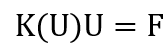
In Abaqus, convergence refers to the successful solution of the finite element method equations:
![]()
The “K” is the stiffness matrix, the “U” is called the displacement matrix, and the “F” is the force matrix (see figure 1 as an example). When this equation is solved correctly, we will have accurate results, and here we use the term “the problem is convergence”. If by any means the equation cannot be solved or has some issues which give us inaccurate results, we use the term “there are some FEA convergence issues or convergence problems.”
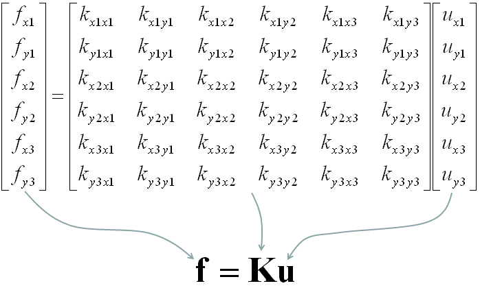
Figure-1 an example of a stiffness matrix with the dimension 6×6
2.1. Different convergence meanings in FEA
In FEA “convergence” can imply multiple meanings such as:
- Mesh convergence
- Time integration accuracy
- Convergence of nonlinear solution procedure
- Solution accuracy
You may wonder what are these meanings and at first sight of talking about, you always address ‘Mesh convergence’ but as you can see, we have four different meanings for convergence that are going to be introduced.
2.1.1. Mesh convergence
The solution of FEA is highly dependent on mesh size and the type of elements. It is important that you use a sufficiently refined mesh to ensure that the results from your Abaqus simulation are adequate. The mesh is said to be converged when further mesh refinement produces a negligible change in the solution.
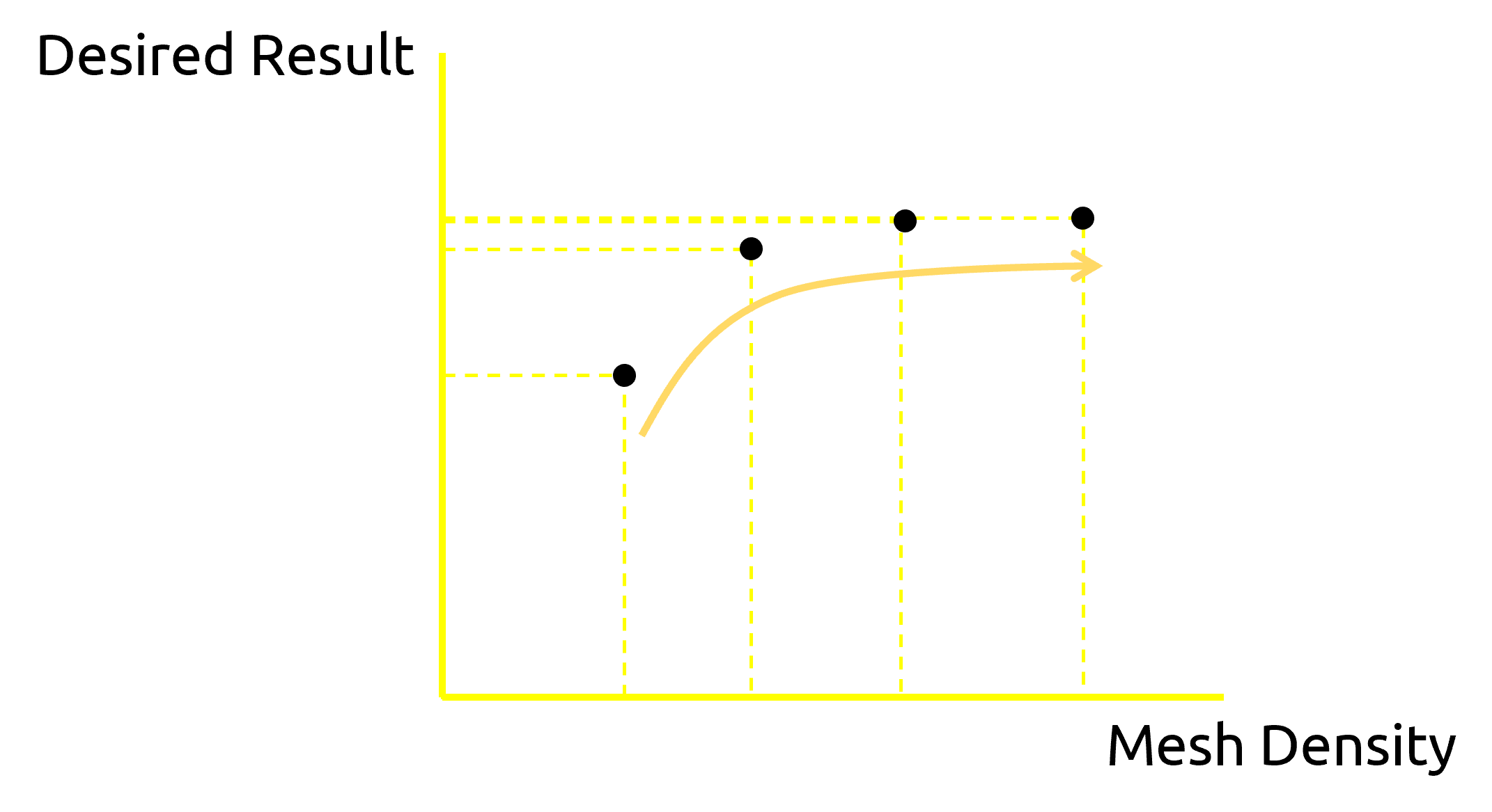
Figure 2: An example of obtaining Mesh convergence
For any simulation in Abaqus, you need to implement a mesh convergence study to ensure your results are converged so they are accurate and reliable in the aspect of mesh.
To perform a mesh convergence study, follow these steps:
- Start by creating a mesh with the smallest reasonable number of elements and analyze your model.
- Increase the mesh density by adding more elements, analyze the model again, and compare the new results with the previous ones.
- Continue this process, increasing the mesh density and re-analyzing until the results show satisfactory convergence.
You don’t need to refine the entire model mesh because this will increase the overall computational cost. You may refine the mesh in some areas of interest that you have identified as the critical areas of your analysis.
For this purpose, you can also use “Abaqus adaptive remeshing” which provides an automated process to remesh your model adaptively. The goal of the adaptive remeshing process is to approach or reach targets on selected error indicators for a specified model and its accompanying load history.
Not only the mesh size but also the element types you use for your model can cause convergence issues. In order to get more familiar with meshing techniques in Abaqus, we recommend to read the following article:
Mastering the Abaqus Mesh: A Guide to Meshing Techniques in Abaqus
2.1.2. Time integration accuracy
The size of the time increment is an important factor for solution convergence especially when the problem is transient and has a physical time scale. Abaqus/Standard provides tolerance parameters to indicate the level of accuracy required in the approximate time integration.
The following tolerance parameters are available for specific analysis procedures:
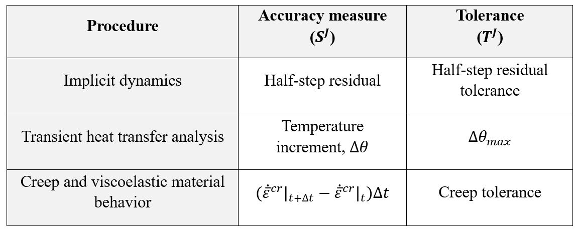
Figure 3: Defining tolerance parameters for time integration
In any transient analysis where automatic time incrementation is used, some of these tolerances, ![]() , will be active. Corresponding measures of the integration accuracy,
, will be active. Corresponding measures of the integration accuracy, ![]() , will be calculated for each increment in the step. Abaqus/Standard will use these values to adjust the time incrementation using the criteria described in this section. The smallest time increment required by all criteria is used if more than one accuracy measure is active.
, will be calculated for each increment in the step. Abaqus/Standard will use these values to adjust the time incrementation using the criteria described in this section. The smallest time increment required by all criteria is used if more than one accuracy measure is active.
For any control, J, that is active in the step, if the time increment is too large to satisfy that time integration accuracy requirement, the increment is therefore begun again with a time increment of:
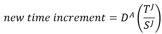
where you can define the value of ![]() . By default,
. By default, ![]() .
.
The half-step residual ![]() is the equilibrium residual error (out-of-balance forces) halfway through a time increment. If the half-step residual is small, it indicates that the accuracy of the solution is high and that the time step can be increased safely; conversely, if the half-step residual is large, the time step used in the solution should be reduced.
is the equilibrium residual error (out-of-balance forces) halfway through a time increment. If the half-step residual is small, it indicates that the accuracy of the solution is high and that the time step can be increased safely; conversely, if the half-step residual is large, the time step used in the solution should be reduced.
You can define the half-step residual tolerance manually when you define a “Dynamic Implicit” step, in the ‘Incrementation’ tab as shown in figure 4.
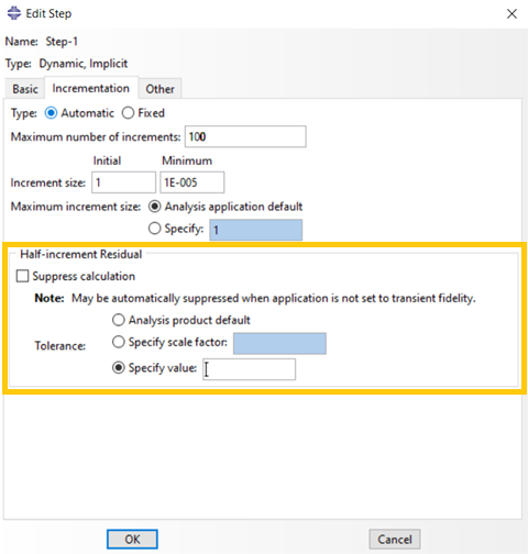
Figure 4: Defining half-step residual tolerance
- If
 high accuracy
 - If
 moderately good accuracy
 - If
 time stepping is rather coarse
( ![]() is a typical magnitude of real forces in an undamped elastic system).
is a typical magnitude of real forces in an undamped elastic system).
Time incrementation in a transient heat transfer analysis can be controlled directly by you or automatically by Abaqus/Standard. Automatic time incrementation is generally preferred. The time increments can be selected automatically based on the user-prescribed maximum allowable nodal temperature change in an increment, ![]() .
.
You can define the maximum allowable temperature change per increment manually when you define a “Heat Transfer” step, in the ‘Incrementation’ tab as shown in figure 5.

Figure 5: Defining the maximum allowable temperature change per increment
Abaqus/Standard monitors the stability limit automatically during explicit integration. At any point in the model, if the creep strain increment is larger than the total elastic strain, the problem will become unstable and Abaqus will calculate a new smaller stable time step.
You can define the creep tolerance manually when you define a “Visco” step, in the ‘Incrementation’ tab as shown in figure 6.
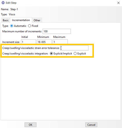
Figure 6: Defining the creep tolerance
2.1.3. Convergence of nonlinear solution procedure
Nonlinear problems arise frequently in various fields of science, engineering, and mathematics. These problems exhibit complex behavior due to the nonlinear relationships between variables. One of the fundamental challenges in dealing with nonlinear problems is ensuring the convergence of proposed solutions.
In the case of nonlinear problems, iterative numerical techniques must be used in order to achieve the solution. The general form of a nonlinear equilibrium equation is:
As you can see the stiffness matrix is also dependent on the displacement values which must be found as the solution. So, numerical methods like Newton-Raphson must be implemented to find the solution. The linear and nonlinear problems will be discussed in the next. A schematic of finding the solution of a nonlinear problem is shown in figure 7 using the “Direct” method.
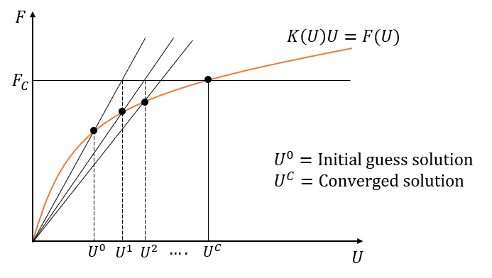
Figure 7: Convergence of a nonlinear problem
2.1.4. Solution accuracy
Accuracy refers to how close a measurement is to the true value. An accurate solution requires all the mentioned convergence terms including:
- Converged mesh
- Accurate time integration for transient problems
- Proper convergence for nonlinear solution procedure
- In addition, an accurate solution requires good engineering judgment to create a proper finite element model, including materials, loads, boundary conditions, and solution procedures
3. Symptoms for the ABAQUS convergence issues
Now, how do we know there is a FEA convergence issue? You could see the solving procedure when running a job by clicking on the “monitor.” As you see (figure2), there are “Error” and “Warning” tabs. You can see some messages that inform you about your issues. Also, you could find more information in “.msg” (Standard solver), “.dat,” and “. sta” (Explicit solver) files. These convergence problems are more in nonlinear models than the linear ones. Some examples of these symptoms are shown in figure 8.
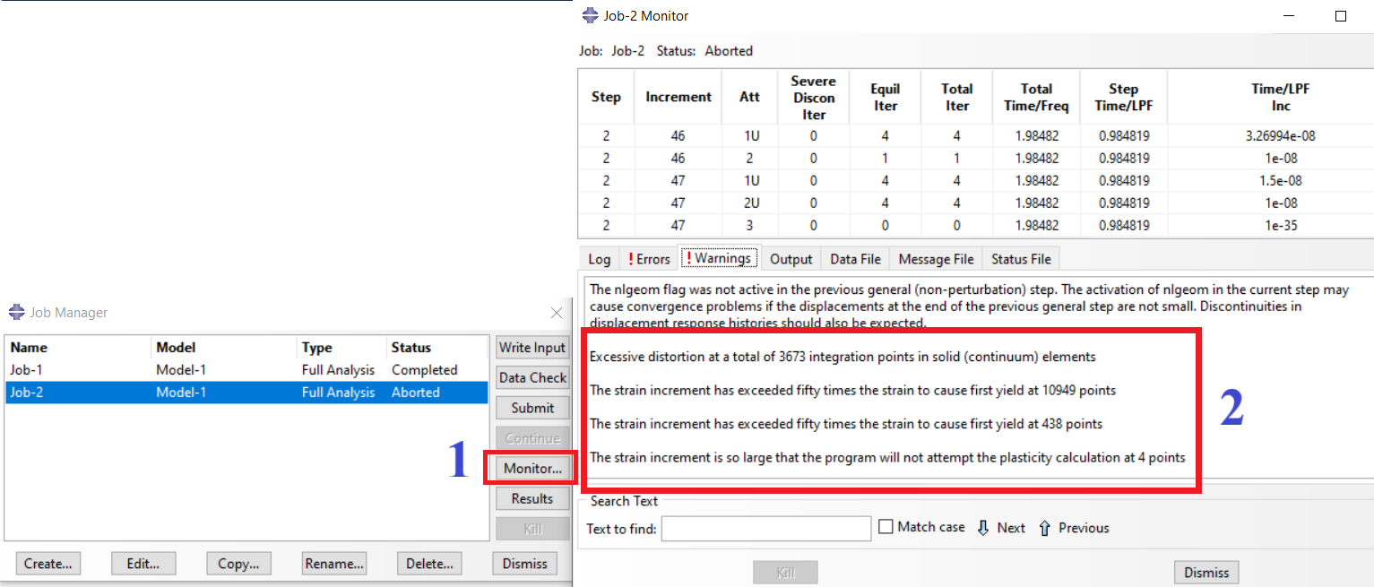
Figure-8: some warnings in the monitor window / Abaqus convergence problem
4. Why we face with ABAQUS convergence issues? | Abaqus convergence problem
This section will explain the reasons for the ABAQUS convergence issues or Abaqus convergence problems. It may be more than we explain here, but we discussed the most important and common ones.
Incomplete and defective modeling in FE is the most common reason for convergence issues; for example:
- Defining inappropriate constraints that cause conflicts in boundary conditions or contact conditions.
- Using wrong elements.
- Defining inadequate material in the property module.
- Defining inappropriate boundary conditions or contacts that may lead to Abaqus contact convergence issues.
- Modeling an unstable physical system.
- Setting an improper increment size can lead you further away from resolving FEA convergence problems.
Now, we intend to explain one or two of these conflicts that lead to Abaqus convergence issues. See figure 9 for an example. Imagine you have a box, and an amount of pressure is applied to it. You want to calculate the stress; if you do not define the boundary condition, the box moves, and the software cannot calculate the stress, and you will see an error. Note that this only happens when you analyze a static problem and use the Static step. Another example is if you constrain a surface and apply pressure on it simultaneously (see figure 10), the software will show an error; because it is not possible to have the surface fixed and apply pressure at the same time (inappropriate boundary conditions). usually these errors are called “Zero Pivot Errors“.
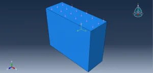
Figure-9: pressurized box without boundary conditions
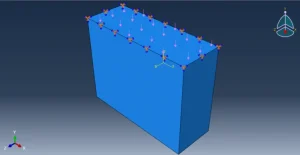
Figure-10 inappropriate boundary conditions

5. Identifying ABAQUS convergence issues
Here, we intend to present some recommendations to identify which symptoms and reasons are causing the issues, the “Errors” and the “Warnings.” The general way is to list the top potential reasons and then check them to see the changes in the software. In the end, start to fix them one at a time. Now, here are some of our recommendations:
5.1. One of the best ways is to simulate a simpler model:
- If possible, make a 2D model or a linear one to have fewer details and elements.
- If possible, do not enter Plasticity or Nonlinear geometry to understand the model’s behavior.
- In a model with several pieces, insert one piece at a time to minimize the number of FEA convergence problem sources.
5.2. Set increment values
Set appropriate increment values that include initial increment, minimum increment, maximum increment size, and the maximum number of increments. To learn more about increments, click here.
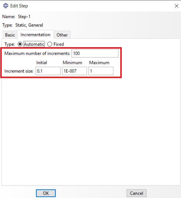
Figure-11 Static general step window and Incrementation tab
When the ABAQUS standard solver starts to run a Job, it splits the step in the maximum number of increments you specified (system default is 100). According to the specified increment size (Figure 11), the solver starts to run the Job. In the case of increments in the ABAQUS Standard solver, you typically encounter three errors that often indicate an ABAQUS convergence problem:
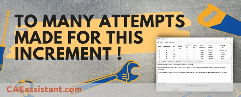
“Too many attempts made for this increment“; means the solver attempted several times to calculate the equations for this increment, but the FEA convergence conditions were not satisfied; click to see how to solve this error: Too Many Attempts Made for This Increment Abaqus error | Why and Solution
“Too many increments needed to complete the step“; means the solver needs more increments; therefore, you have to increase the “Maximum number of increments” until you overcome this convergence problem.
“Time increment required is less than the minimum specified“; in this Error, you have to decrease the “Minimum” in “Increment size” to satisfy the convergence conditions.
The error “Time increment required is less than the minimum specified” in Abaqus typically occurs when the solver determines that a smaller time increment than the specified minimum is necessary to maintain solution accuracy or stability. This could be due to highly nonlinear behavior, such as contact changes or material nonlinearity, requiring finer increments for convergence.
Read More: Abaqus tutorial PDF & video
5.3. See the reasons for FEA convergence issues
See the reasons for convergence issues reported in the .dat, .sta, .msg, and .odb files.
You can add more information in the message files. For example, use the keyword command “*PRINT, CONTACT=YES” in the input file of the model (-.inp) to get contact information in the message file. This could help you to find out the ABAQUS contact convergence problems. Also use the command “*PRINT, PLASTICITY=YES” to get the integration point numbers and element output for material issues. You can use the “*PRINT” command to add more information in message files (.msg, .sta). Be patient, and we will explain to you how to use this command.
First, you need to know the input file (.inp). The Input file is one of the ABAQUS files that contains model data such as load, step, etc. It is like the “.cae” file but has less size, and you can open it in a text file and change whatever you want. When you have created your model completely and then created a Job for it, before you run it, you can create an input file for the model by clicking on the “Write Input” button in the “Job Manager” window (see figure 12). You can open the input file in a text file and change whatever you want; then, to use it in the ABAQUS, open the file according to Figure 13.
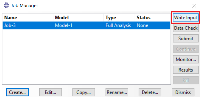
Figure 12 Create an input file
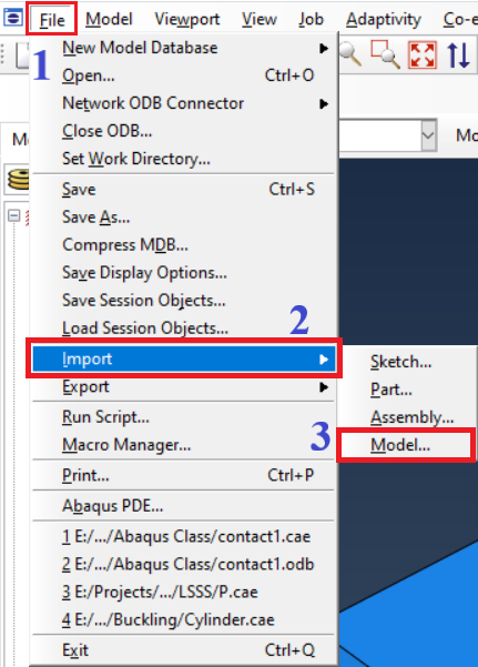
Figure 13: Open the Input file in the software
Now, as you know what an input file is, let’s use the “*PRINT” command. You can find the instructions about the “*PRINT” command or any other keywords in the Keywords in the ABAQUS documentation (Figure 14).
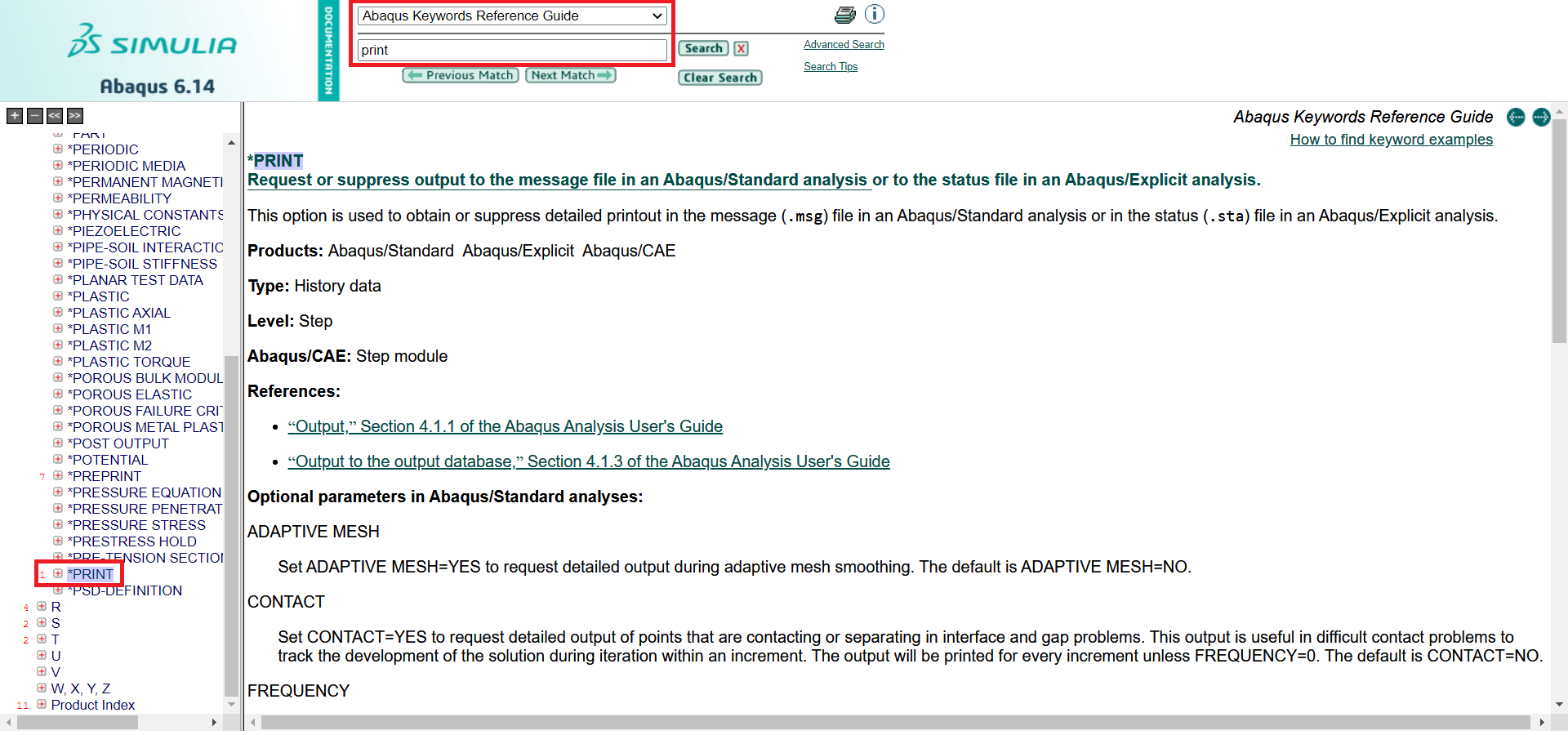
Figure 14 Finding PRINT keyword in ABAQUS documentation
As you can see in Figure 15, open your input file through the Edit Keywords window; then, find the lines that define the loading conditions; after these lines and before “*END STEP,” you can add your “*PRINT” commands then click OK button. After running the Job, you would see the results in the .msg (Standard solver) and .sta (Explicit solver) files. Now, you know how to write an input file, use it, and modify it.
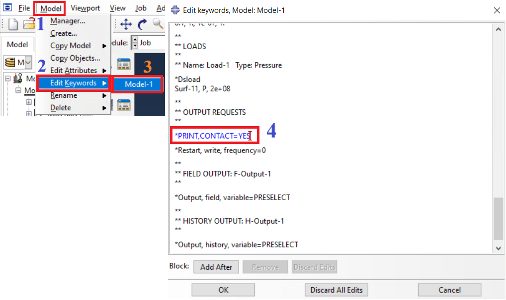
Figure 15 Enter the PRINT command
5.4 Contact Convergence Problems and Contact Definition
There are two main reasons why contact issues can lead to non-convergence in Abaqus simulations: Abaqus contact convergence
- Unstable Contact: Contact itself can introduce instabilities into your model. Imagine two rigid surfaces grinding against each other. This kind of interaction can cause large, abrupt changes in the forces acting on the parts, which can be difficult for Abaqus to solve for numerically.
- Incorrect Contact Definition: If you don’t define the contact between parts properly, it can lead to unrealistic behavior in your model. For instance, you might forget to define contact for surfaces that are supposed to be touching, or you might use the wrong contact formulation for the type of interaction you’re simulating. This can lead to forces that are too large or too small, or even to parts passing through each other, all of which can cause convergence problems.
Here are some ways to address these issues:
- Contact Stabilization: Abaqus offers contact controls that can help to stabilize the solution during the analysis.expand_more These controls can include things like friction dissipation and penalty stiffness scaling.expand_more
- Refining the Mesh: A finer mesh can sometimes help to improve the accuracy and stability of the contact solution. This is because a finer mesh allows for a more accurate representation of the contact surface.
- Verifying Contact Properties: Double-check that you have defined the contact properties correctly, including the type of contact, the surfaces that are in contact, and any relevant friction or adhesion coefficients.
By carefully considering these factors, you can improve your chances of achieving convergence in your Abaqus simulations that involve contact.
5.4.1 What is a normal contact between two surfaces that have usual contact in real without any penetration? tell me how can I define it in Abaqus?
In Abaqus, normal contact between two surfaces that touch in real life without penetration is typically defined using the general contact interaction property. This property allows for separation (opening) and closure (compression) between the surfaces. Here’s how to define it:
- Surface Definition:
First, you need to define the surfaces that will be in contact. Abaqus offers several options for defining surfaces, such as:
- Element-based surfaces: This is the most common approach. You can select specific faces of elements (nodes) to create the contact surface.
- Node-based surfaces: You can directly select individual nodes to define the contact surface.
- Interaction Property:
- In the Interaction module of Abaqus/CAE, create a new interaction property.
- Select “General Contact” as the interaction type.
- Assign a name to the interaction property.
- Contact Properties:
- Normal Behavior:
- Choose “Hard Contact” for the normal behavior. This option prevents the surfaces from penetrating each other.
- You can optionally define a pressure-overclosure relationship to model more complex contact behavior.
- Tangential Behavior:
- By default, Abaqus assumes frictionless contact.
- You can define a friction coefficient if there is friction between the surfaces.
- Abaqus offers various friction models like penalty friction or exponential decay friction.
- Other Options:
- You can adjust various other options within the general contact definition, such as surface smoothing or contact stiffness scaling, to improve convergence or refine the contact behavior.
- Assigning the Interaction:
- Once you have defined the contact property, assign it to the set of surfaces that will be in contact.
In the video below, you can familiarize yourself with the interaction module and how to define contact.
In this post, we have attempted to address ABAQUS convergence problems. We have explored how the finite element method relies on a primary equation, and when this equation remains unsolved, leading to an FEA convergence problem. Additionally, we have discussed the symptoms of ABAQUS convergence issues, why we encounter them, methods for identifying ABAQUS convergence problems, and the reasons behind FEA convergence problems.
We, the CAE Assistant team, hope you have got enough information about the Abaqus convergence problem and Abaqus contact convergence issues in this post. The upcoming articles will focus on tools and methods for resolving Abaqus errors, particularly convergence issues. You can click on “Debugging of ABAQUS errors” for more information.
Please share your views with us in the comment section. We really appreciate your feedback, as it helps us improve our tutorials and fulfill all your CAE needs without requiring additional tutorials. It would be useful to see Abaqus Documentation to understand how it would be hard to start an Abaqus simulation without any Abaqus tutorial. Additionally, you can obtain a PDF version of this post to review the FEA convergence problem by clicking on “Abaqus convergence issues PDF.”
|
⭐⭐⭐Free Abaqus Course | ⏰10 hours Video 👩🎓+1000 Students ♾️ Lifetime Access
✅ Module by Module Training ✅ Standard/Explicit Analyses Tutorial ✅ Subroutines (UMAT) Training … ✅ Python Scripting Lesson & Examples |
Reference: Troubleshooting Finite-Element Modeling with Abaqus
6. Users ask these questions
Now, let’s see some common questions that users ask and we tried to answer them as best we could.
I. Displacement control or Load control
Q: Which one is the better axial displacement or concentrated force in tensile loading in Abaqus analysis?
A: In pure tension, it’s better to use Displacement instead of Force; because it will minimize convergence problems, and iterating a solution is better controlled. If the analysis is a pure bending, instead of Moment, use a Displacement/Rotation instead of a concentrated moment load.
| ✅ Subscribed students | +80,000 |
| ✅ Upcoming courses | +300 |
| ✅ Tutorial hours | +300 |
| ✅ Tutorial packages | +100 |
What are the reasons behind the Abaqus convergence issues?
The most important reasons for convergence issues are:
- Defining inappropriate constraints that may cause conflicts in boundary conditions or contact conditions.
- Using wrong elements.
- Defining inadequate material in the property module.
- Defining inappropriate boundary conditions or contacts.
- Modeling an unstable physical system.
- Set an improper increment size.
What does convergence in Abaqus mean?
The finite element method uses this main equation to solve a problem: F=K×U. The “K” is the stiffness matrix, the “U” is called the displacement matrix, and the “F” is the force matrix. When this equation is solved correctly, we will have accurate results, and here we use the term “the problem is convergence”.
What should we do when faced with a convergence issue?
- First, check all boundary conditions, contact conditions, material properties, and load conditions.
- Then, in a model with several pieces, insert one piece at a time to minimize the number of issues sources.
- If the convergence problem is not solved, try to simulate a simpler model by making a 2D model or don’t use the plasticity property in material behavior. Also, see the reasons for convergence issues reported in the (.dat), (.sta), (.msg), and (.odb) files.
What is the error “Too many attempts made for this increment”?
Read this article to find out: “Too many attempts made for this increment”.
How can I extract the reasons for convergence issues in the .sta and .msg files?
You can use the “*PRINT” command to add more information in message files (.msg,. sta). First, open the input file and add your desired “*PRINT” commands; then, run the input file. After running the job, you will see the results in the .msg (Standard solver) and .sta (Explicit solver) files.
Thank you for being with us in this article. In order to always provide you with up-to-date and engaging content, we need to be familiar with your educational and professional experiences so that we can offer articles and lessons that are most useful to you.