
Increasing load rate in an Abaqus quasi static analysis
A lot of Abaqus users face a common problem: their analyses, especially the quasi static analysis, take a really long time to finish. This can be quite annoying. Fortunately, there are two methods to speed up these Abaqus quasi static analysis: one is using “Abaqus mass scaling,” and the other is increasing the “Abaqus load rate.” In this post, we’ll concentrate on the latter method, which involves making your analyses faster by adjusting the load rate. We’ll also guide you on how to determine which load rate is suitable for your quasi static analysis in Abaqus.
Quasi static problems are one of those that usually would be solved with Abaqus/Standard but may have difficulty converging because of contact or material complexities, resulting in a large number of iterations. Challenging nonlinear quasi-static problems often involve:
* Very complex contact conditions, which Abaqus/Standard may fail to converge due to contact issues.
** Very large deformations that can lead to severe mesh distortion.
For example, typically, in metal forming analysis, we face such difficulties:
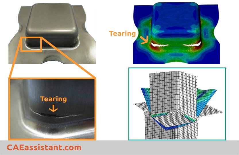
Example: Simulation of tearing in a deep drawing process
It is really hard to model such a problem with Abaqus/Standard.
 |
⭐⭐⭐Free Abaqus Course | ⏰10 hours Video 👩🎓+1000 Students ♾️ Lifetime Access
✅ Module by Module Training ✅ Standard/Explicit Analyses Tutorial ✅ Subroutines (UMAT) Training … ✅ Python Scripting Lesson & Examples |
For forming process, we have these video tutorial packages:
 |
|
 |
|
Quasi static analysis in Abaqus/Explicit Problems
Abaqus/Explicit is more efficient for modeling highly nonlinear static (quasi-static analysis) problems. This is especially true for three-dimensional problems involving contact and very large deformations like metal forming.
Application of Abaqus/Explicit to model quasi-static events requires special consideration. It is computationally impractical to model the process in its natural time period. Literally, millions of time increments would be required. Therefore, we artificially increase the speed of the process in the simulation to obtain an economical solution.
| If you would like to know more about Abaqus/Standard and Abaqus/Explicit, we’ve already covered the differences between them in this article titled, Abaqus/Standard or Abaqus/Explicit? | Abaqus Dynamic Explicit |
Two approaches to obtaining economical Abaqus quasi-static analysis solutions are:
1. Increasing Abaqus Load Rates
We can artificially reduce the time scale of the process by increasing Abaqus loading rate. Increased load rates reduce the time scale of the simulation, so fewer increments are needed to complete the job.
Increasing load rates by a factor of f, increases the analysis speed by a factor of f.
2. Mass scaling
It increases the size of the stable time increment, so fewer increments are needed to complete the job. Artificially increasing the material density (mass scaling) by a factor of f2 increases the analysis speed by a factor of f.
In this article, our focus is on increasing Abaqus load rates.
To reduce the number of require increments in an quasi static analysis in Abaqus/Explicit, we can speed up the simulation compared to the time of the actual process—that is, we can artificially reduce the time period of the event or, equally, increase the rate of loading. This will introduce possible errors. If the loading rate is increased too much, the increased inertia forces will change the predicted response. In an extreme case, the problem will exhibit a wave propagation response. The only way to avoid this error is to choose a load rate that is not too large.
Finding out Abaqus load rate is appropriate or not
As discussed, there are two options to reduce the computational cost of quasi-static analysis: mass scaling and increasing the load rate in Abaqus. When utilizing the Abaqus mass scaling feature, the system’s mass is multiplied by a factor. While it can reduce computational costs, high mass scaling coefficients may significantly affect results. Moreover, increasing the load rate in Abaqus can lead to a dynamic response rather than the quasi-static Abaqus solution. Therefore, both techniques must be used with care. Various criteria have been provided to check if quasi-static analysis in Abaqus is performed with sufficient accuracy.
1) Running several simulations with different load rates
- Run a series of simulations in the order from the fastest load rate to the slowest. As you know, the analysis time is greater for slower Abaqus load rates.
- Examine the results (deformed shapes, stresses, strains and energies) to get an understanding of the effects of varying the model when changing the load rate Abaqus:
»Excessive tool speeds in sheet metal forming tend to promote unrealistic localized stretching.
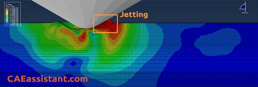
»Excessive tool speeds in bulk forming simulations cause jetting (hydrodynamic-type response).
 »Excessive loading rates can cause highly localized deformation near the applied load.
»Excessive loading rates in an Abaqus quasi-static collapse analysis can result in a steep initial slope of the load versus displacement curve due to increased (non-structural) resistance to initial deformation. Sometimes, localized buckling may occur near the applied load.
2) Using natural frequency to check the Abaqus load rate
The dominant response of a quasi-static analysis will be the first structural mode. Therefore, we use the frequency of this mode to estimate the proper load rate Abaqus:
- Estimate the first natural frequency (f) of the model. In simple models, we may find this frequency by available analytical relations. For models that are more complex, first, run a Frequency analysis in Abaqus.
- Calculate the corresponding time period (T) using the first natural frequency of the model:
T=1/f
- Run the Explicit analysis (step time=T) and estimate the global deflection (D) in the impact direction of the model during this time (T). (read more about Abaqus Step Time)
- Calculate the impact velocity (V):
V=D/T
- A general recommendation is to limit the impact velocity to less than 1% of the wave speed of the material. Typical wave speed in metals is 5000 m/sec.
Note: If you want to know more about the speed and velocity in Abaqus, read this article: Applying Abaqus Velocity | Angular Velocity VS Linear Velocity
3) Comparison of kinetic and internal energies in quasi-static analysis
To ensure quasi-static behavior, especially when increasing the load rate or defining a mass scaling factor in an explicit step within Abaqus, you can compare kinetic and internal energies. This helps verify that the mass scaling factor and the load rate in Abaqus are sufficiently small. For those interested in the practical implementation of this approach, it is discussed in the following section.
In quasi-static analysis, it is crucial to keep the kinetic energy of deformable bodies below a critical percentage of the total internal energy. The Abaqus documentation recommends maintaining this critical range between 5 and 10 percent. We will now explain how to check this criterion in your simulation.
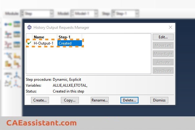
When defining a dynamic explicit step in Abaqus, the energy for the entire system is automatically extracted in the form of history outputs. To examine this process, create a dynamic explicit step in the ‘Step’ module and then click on the ‘History Output Manager’ icon. As shown in the next figure, Abaqus automatically generates a history output for the explicit step.
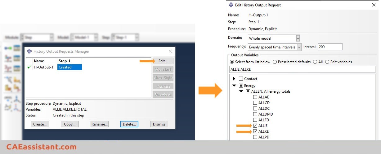
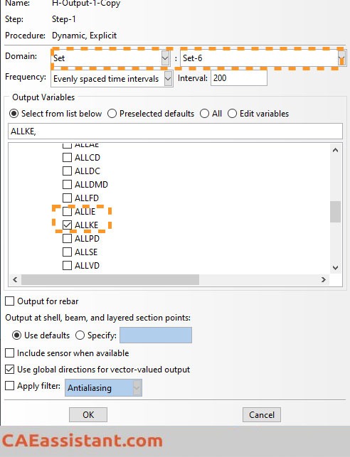
You can edit the created history output and deselect unnecessary results. For example, as illustrated in the next figure, we have unchecked all energy components except ALLIE and ALLKE. They represent the total internal energy and kinetic energy, respectively.
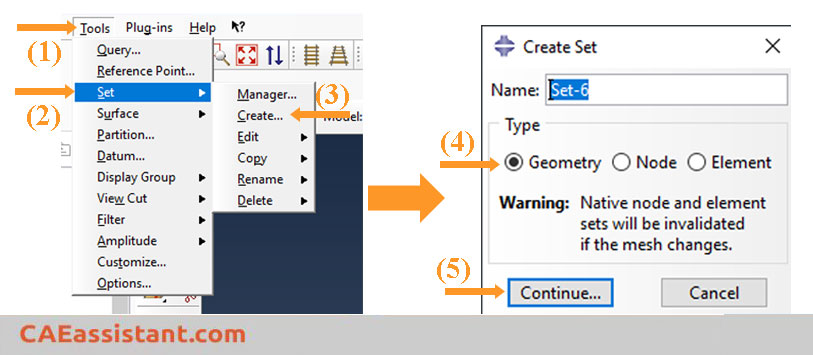
Note that the kinetic energy chosen in the ‘Edit History Output Request’ window includes the energy for the rigid bodies. However, if your model has rigid bodies with assigned mass, you must subtract the kinetic energy for rigid bodies from the total kinetic energy. To achieve this, start by creating a set that includes all rigid bodies with mass. To do so, navigate to the ‘Step’ module, click on ‘Tools’, then select ‘Set’, and finally, click on ‘Create’. Choose ‘Geometry’ for the type and click ‘Continue’. The procedure is illustrated in the following figure.
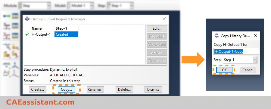
Now, choose the rigid bodies in the model and click ‘Done’. Next, click on the ‘History Output Manager’ icon, and copy the existing history output, as illustrated in the next figure. Finally, click ‘OK’ to generate the history output.
Next, in the ‘History Output Manager’ window, select the second history output and click ‘Edit’. As shown in the next figure, choose ‘Set’ from the ‘Domain’ combo box, then select the set that includes rigid bodies (e.g., Set-6 in the figure). Uncheck ALLIE since it is not needed, and click ‘OK’ to proceed. Abaqus will now extract the kinetic energy for rigid bodies.
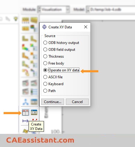
Now, assume that you have submitted the job, and it is completed. You want to check the solution to determine whether the load rate in Abaqus is sufficiently small to access a quasi-static solution or not. To do so, go to the visualization module, click on the ‘Create XY Data’ icon, and then ensure that the ‘ODB history output’ is chosen. Finally, click ‘Continue’. The procedure is presented in the following figure.

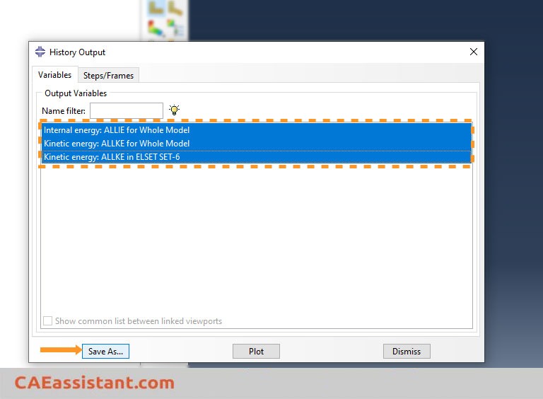
Afterward, select the internal and kinetic energies, as shown in the following figure, and click on ‘Save as’. Note that if you have no rigid body in your model, you only need to choose the total internal and kinetic energies. Otherwise, the kinetic energy for the rigid body must also be selected.
In the displayed window, choose ‘As is’ and click ‘OK’. If you have rigid bodies with assigned mass in your model, click on the ‘Create XY Data’ icon, and then select ‘Operate on XY data’. Click ‘Continue’ to proceed.
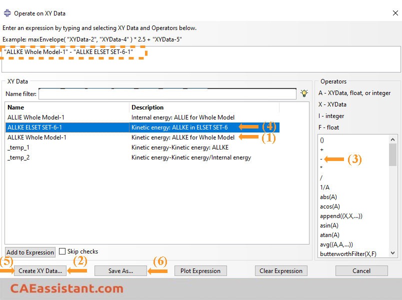
Now, select the total kinetic energy and click ‘Add to expression’. Then, click on the minus sign and choose the kinetic energy for the rigid bodies. Once more, click ‘Add to expression’ and then click ‘Save as’. The procedure is illustrated in the following figure.
Choose a name for your data and save it. Note that the saved data is the total kinetic energy minus the energy of rigid bodies. Click the ‘XY Data Manager’ icon, and select both the operated data and the total internal energy. If your model has no rigid bodies with assigned mass, choose the total kinetic energy instead of the operated data. Finally, click ‘Plot’.
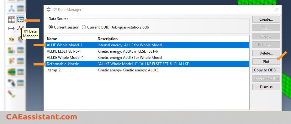
Now you have plotted the internal and kinetic energies, as shown in the following figure. So, you can compare their ratio to determine if the load rate in Abaqus is sufficiently small to indicate a quasi-static solution or not.
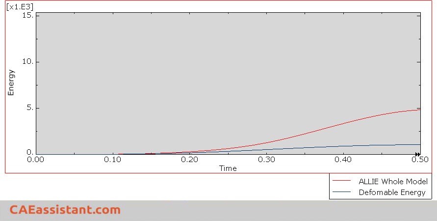
Moreover, you can click on the ‘Create XY Data’ icon and select ‘Operate on XY Data’. Next, divide the kinetic energy by the total internal energy to check if the ratio is below 10 percent. If the ratio exceeds the critical value, you can either decrease the mass scaling factor or adjust the load rate in Abaqus.
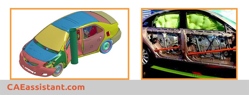
Example (Door Beam Intrusion Test)
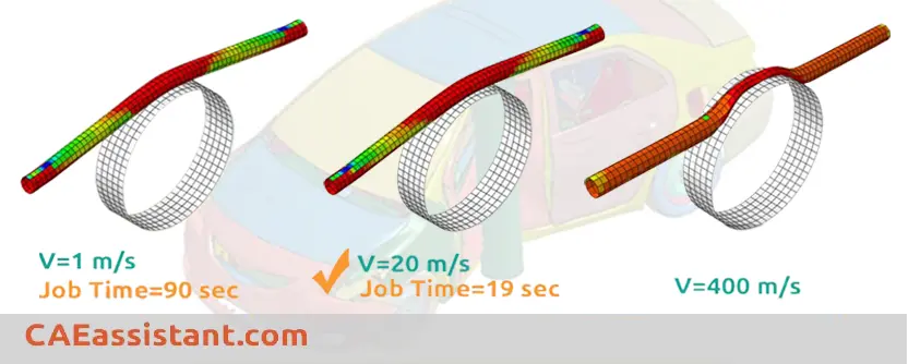
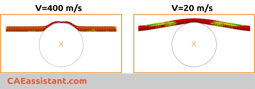
To illustrate the problem of determining the proper loading rate, consider the deformation of a side intrusion beam in a car door. This test falls into the category of Abaqus quasi-static analysis
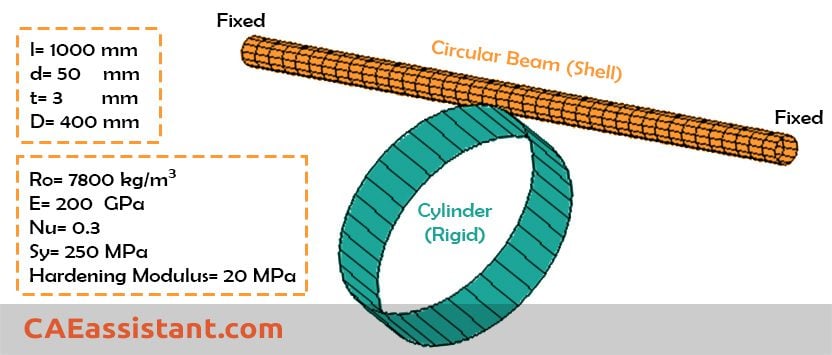
 We model the test as the circular beam (length of l, diameter of d and thickness of t) is fixed at each end, and a rigid cylinder (diameter of D) deforms the beam.
 Here, we check the velocity of 20 m/s and 400 m/s for a cylinder to see which one can be applicable to our problem.
- The frequency of the first mode is approximately 250 Hz: f=250
- This rate corresponds to a period of 4 milliseconds: T=1/250=0.004 s
- Using a velocity of 20 m/sec, the analysis shows cylinder will be pushed into the beam 0.1 m in 4 milliseconds: D=0.1 m
- The impact velocity is:
V=D/T= 0.08/0.004= 20 m/s
- Recalling the wave speed in metals is about 5000 m/sec, so the impact velocity 25 m/sec is about 0.5% of the wave speed (less than 1%).
If we check the velocity of 400 m/s it will result in about 4% of wave speed (unacceptable).

Limitations
i. As the speed of the process is increased, a state of static equilibrium evolves into a state of dynamic equilibrium and inertia forces become more dominant. We should try to model the process in the shortest time period (largest load rate Abaqus) in which inertia forces are still insignificant.
ii. Some aspects of the problem other than inertia forces—for example, material behavior—may also be rate-dependent. In this case, the actual time period of the event being modeled cannot be changed. The mass scaling approach gets attractive in such problems.
Using Smooth Step amplitude curve
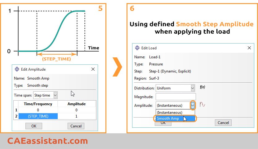
We could obtain a more accurate Abaqus quasi-static solution by applying loads gradually.
By default, Abaqus/Explicit loads are applied immediately and remain constant throughout the step. Instantaneous loading may induce the propagation of a stress wave through the model, producing undesired results. For instance, constant velocity boundary conditions result in a sudden impact load onto a deformable body.
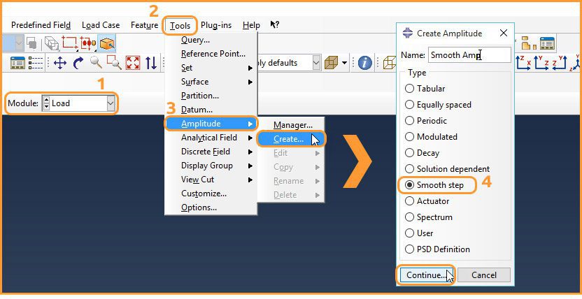
We can ramp up (or down) the loading gradually from (to) zero by defining a smooth step amplitude in an Abaqus quasi-static solution:
What is quasi-static analysis?
In summary, in quasi-static analysis, the assumption is made that the problem can be treated as static at any specific moment in time. The key concept is that the applied loading changes very gradually, with a frequency significantly lower than that of the structure. As a result, the structure deforms as if it were under static conditions, and the influence of inertia is considered negligible. This assumption is effective when the effects of inertia are minimal, and it allows for the simplification of non-linear problems into linear systems.
In long term, Quasi-static analysis is a method used in engineering and physics to analyze the behavior of a system or structure under slowly varying loads or conditions. It is a simplified approach that assumes the system remains in equilibrium at each stage of the analysis, neglecting the dynamic effects and considering only the static forces.
In quasi-static analysis, the system is divided into a series of static equilibrium states, and the response of the system is determined at each step. The applied loads are assumed to change gradually or incrementally, allowing the system to adjust and reach a new equilibrium at each stage. This analysis technique is often used when the dynamic effects, such as inertia, vibration, and time-dependent behavior, can be considered negligible compared to the static forces and deformations.
Quasi-static analysis is commonly employed in various fields, including structural engineering, mechanical engineering, civil engineering, and materials science. It helps engineers and researchers understand how a structure or system will respond under various loads and allows for the calculation of stresses, strains, displacements, and other relevant parameters. By simplifying the analysis to static equilibrium states, it provides a practical and efficient approach for predicting the behavior of systems subject to slow or gradual changes.
Difference between quasi-static analysis and dynamic analysis
The main difference between quasi-static and dynamic analyses lies in the consideration of time-dependent effects and the assumption of equilibrium.
Quasi-static analysis assumes that the system or structure remains in equilibrium at each stage of analysis and neglects the dynamic effects such as inertia, vibration, and time-dependent behavior. It is suitable for situations where the time scale of the loading or the response is much larger than the characteristic time scale of the dynamic effects. Quasi-static analysis is computationally simpler and often provides a reasonable approximation for slowly varying or static loads.
On the other hand, dynamic analysis explicitly accounts for the time-dependent behavior of a system or structure. It considers the effects of inertia, damping, and time-varying forces. Dynamic analysis is necessary when the time scale of the loading or the response is comparable to or larger than the characteristic time scale of the dynamic effects. It is used to study the behavior of structures subjected to rapid or impulsive loads, seismic events, vibrations, and other dynamic phenomena.
While quasi-static analysis is simpler and computationally less demanding, dynamic analysis provides a more accurate representation of the system’s behavior under time-varying conditions. However, there are cases where a combination of both approaches is needed.
In dynamic analysis, there are situations where quasi-static analysis is used as part of the overall analysis. This can occur when the dynamic response is dominated by certain frequencies or modes of vibration. In such cases, the dynamic analysis may be separated into two parts: a quasi-static analysis to determine the response at low frequencies or during initial stages, and a dynamic analysis to capture the higher-frequency or time-dependent behavior. For example, in seismic analysis of structures, a quasi-static analysis may be performed to evaluate the response under the predominant low-frequency ground motions, followed by a dynamic analysis considering the higher-frequency components and the interaction between the structure and the ground.
Abaqus quasi static analysis
How can I know my simulation is quasi-static or not?
As a rule of thumb, a simulation is static or quasi-static if the excitation frequency is less than 1/10 of the lowest natural frequency of the structure. This is mentioned in Abaqus Documentation:
“It is usually desirable to increase the loading time to 10 times the period of the lowest mode to be certain that the solution is truly quasi-static.“
In a static or quasi-static analysis, the lowest mode of the structure usually dominates the response. Therefore, knowing the frequency and, correspondingly, the period of the lowest mode, you can estimate the time required to obtain the proper static response. The natural frequencies can be calculated easily using the eigen frequency extraction procedure in Abaqus/Standard (Frequency analysis).
It would be useful to see Abaqus Documentation to understand how it would be hard to start an Abaqus simulation without any Abaqus tutorial. If you want to get complete information about load rate and mass scaling methods, watch the below demo video of the Abaqus course for beginners package:
In this post, we completely covered speeding up quasi-static analysis in Abaqus by increasing the load rate. You can now choose the appropriate Abaqus load rate and examine it using the methods we discussed, such as ‘Running several simulations’ and ‘Using natural frequency.’ Additionally, by studying the example provided, you can gain a deeper understanding of Abaqus quasi static problems.
It’s your turn to dive into the article and join our quiz! Don’t forget to check out the ‘Practice Time‘ section; you’re supposed to conduct the intrusion test. Please share your experiences, questions, or any comments you might have with us, The CAE Assistant, your assistant in CAE challenges.”
Quiz Time!
1. Abaqus/standard is not appropriate for metal forming simulation at all. (True/False)
2. Stretching is one of the bulk metal forming processes in which Abaqus/explicit is more efficient to simulate. (True/False)
3. We artificially increase the time scale of the process by increasing the Abaqus loading rate. (True/False)
4. Jetting is a hydrodynamic-type response when tool speed in bulk forming simulations is excessive happens. (True/False)
5. Mass scaling by a factor of f decreases the computational cost by a factor of √f. (True/False)
6. Increasing load rate by a factor of f decreases the computational cost by a factor of f. (True/False)
7. By default, Abaqus/Explicit apply loads gradually throughout the step. (True/False)
|
⭐⭐⭐Free Abaqus Course | ⏰10 hours Video 👩🎓+1000 Students ♾️ Lifetime Access
✅ Module by Module Training ✅ Standard/Explicit Analyses Tutorial ✅ Subroutines (UMAT) Training … ✅ Python Scripting Lesson & Examples |
Practice Time!
Try to model intrusion tests, one of the Abaqus quasi static problems. you can model based on the information provided about geometry, material, etc. First, conduct a Frequency analysis to find the basic frequency (first mode) of the beam (with given BC). Then, run three Dynamic, Explicit analyses (as shown in the poster of the article) and compare results.
You can have the PDF of this Post by clicking on speeding up quasi static analysis in Abaqus
Also, learn about: Automatic Stabilization Abaqus of Unstable Problems
Users ask these questions
In social media, users ask many questions regarding, static, quasi-static, loading rate, etc. So, we decided to answer a few of them, which you can see below.
I. Can the Explicit solver be used for static problems?
A: The Explicit solver is the best choice for many cases such as impact, blast analysis, drop testing, simulating short-duration dynamic events, high energy, etc. also, it can be used in the static analysis with some considerations. Usually, the Explicit is used in static problems when you have convergence issues. For more information, see this article: “Speeding up quasi static analysis in Abaqus | Increasing Abaqus load rate”
II. Quasi-static analysis
Q: Hello everyone! To simulate cylindrical turning, I’m using Abaqus. The final kinetic energy is always larger than 5% of the internal energy, regardless of how I set the mass scaling factor (16,100,256, etc.). Finally, I remove the mass scaling, which reveals that the kinetic energy is larger than 5% of the internal energy. How can I configure the model to satisfy the 5% requirement? Thanks!
A: Hello,
The kinetic energy might be greater at the beginning of the analysis, and that’s okay. If it’s steel greater then, I recommend increasing the time period.
Speeding up quasi static analysis in Abaqus | Increasing Abaqus load rate
Best luck, friend.
V. Speed up Abaqus Analysis
Q: How to speed up Abaqus analysis?
A: Perhaps you are familiar with this situation: after preparing your model and initiating the simulation, you open the monitor window and find that it remains empty for a longer period of time than you would prefer. You realize that the simulation is taking longer than you had anticipated, and you begin to question whether there are methods to accelerate the process without significantly compromising the precision of the outcomes.
There are several ways to speed up Abaqus analysis, including:
- Reduce the model size: One of the most effective ways to speed up Abaqus analysis is to reduce the size of the model. This can be achieved by removing unnecessary details or simplifying the geometry of the model without compromising the accuracy of the results.
- Use element types wisely: Choosing the appropriate element type for each part of the model can significantly impact the analysis time. Using simpler elements with fewer degrees of freedom can reduce the computational effort required to solve the problem.
- Optimize the mesh: The mesh size and quality can affect both the accuracy and the computational time of the analysis. A too fine mesh can increase the analysis time and memory requirements, while a too coarse mesh can compromise the accuracy of the results. Therefore, optimizing the mesh size and quality can help to speed up the analysis.
- Use adaptive meshing: Adaptive meshing involves automatically refining the mesh in areas where higher accuracy is required while keeping a coarser mesh in areas where lower accuracy is acceptable. This can reduce the overall mesh size and improve the accuracy of the results while minimizing the computational cost.
- Use symmetry: Taking advantage of symmetry in the model can reduce the size of the problem, which can significantly reduce the computational time. For example, if the model is symmetric about a plane, only one-half of the model needs to be analyzed.
- Use parallel processing: Abaqus supports parallel processing, which involves breaking up the analysis into smaller pieces and solving them simultaneously. Using parallel processing can significantly reduce the analysis time, especially for large models.
- Use efficient hardware: Using a high-performance computer or cluster with sufficient RAM and processing power can significantly reduce the analysis time.
- Use mass scaling: Mass scaling is a technique used in Abaqus to adjust the mass of the model during the analysis. Mass scaling may speed up the Abaqus analysis in certain situations, but it depends on the specific problem and the characteristics of the model.
Overall, there are many ways to speed up Abaqus analysis, and the best approach will depend on the specific problem and the available resources. By using a combination of these tips and techniques, you can optimize the analysis settings, reduce the computational time, and improve the accuracy of the results.
| ✅ Subscribed students | +80,000 |
| ✅ Upcoming courses | +300 |
| ✅ Tutorial hours | +300 |
| ✅ Tutorial packages | +100 |
What is a quasi-static analysis?
The quasi-static analysis is a way to study how things behave when they are slowly loaded or changed over time. It is a simplified approach that assumes that the thing being studied remains in balance at each stage of the analysis. This means that the effects of inertia, or how fast the thing is accelerating, are ignored.
What is quasi-static analysis with Abaqus explicit?
Abaqus/Explicit is more efficient for modeling highly nonlinear static (quasi-static analysis) problems. This is especially true for three-dimensional problems involving contact and very large deformations like metal forming.
How to reduce analysis time in Abaqus?
Increasing Abaqus Load Rates:
Artificially reduce the time scale of the process by increasing the Abaqus loading rate.
Mass scaling:
Increases the size of the stable time increment, reducing the number of increments needed to complete the job.
finest post
Some genuinely prize articles on this site, saved to favorites . Kerrill Bondie Bearce
After looking into a handful of the blog posts on your site, I really appreciate your way of writing a blog. I bookmarked it to my bookmark webpage list and will be checking back in the near future. Take a look at my web site too and tell me how you feel. Maddalena Benedetto Brownley