What is Abaqus Contact Damping and how to apply it in Abaqus?

When two parts come into contact in a simulation, things can get unstable quickly. Movements like sliding or bouncing can cause sudden changes that make your model hard to solve. That’s why Abaqus includes contact damping — a built-in way to smooth things out during contact, similar to how a shock absorber works in real life.

This damping doesn’t represent actual material behavior, but it helps the simulation run more smoothly. In Abaqus/Standard, it’s mostly used for tricky situations like snap-through problems or convergence errors. In Abaqus/Explicit, it’s more common and even applied automatically in some cases. But using damping without understanding it can lead to unrealistic results, so it’s important to know how and when to apply it.

In this article, we explain how contact damping works in both Abaqus/Standard and Abaqus/Explicit. You’ll learn how to implement it using the GUI and input files, how to define damping coefficients, and how it compares with contact stabilization. We also cover best practices and common mistakes, so you can apply damping effectively without compromising accuracy.

1. What is Abaqus Contact Damping?

In Abaqus, contact damping refers to a numerical technique employed to control and stabilize contact interactions between surfaces or bodies in a simulation. It involves adding a damping force or resistance at the contact interface, which helps to mitigate instabilities, oscillations, or chatter that may arise due to rapid changes in contact forces or conditions. This damping force is typically viscous in nature, meaning it acts proportionally to the relative velocity between the contacting surfaces.

When two parts touch or slide in a simulation, things can get tricky. Sudden movements or contact changes can cause instabilities. That’s where Abaqus contact damping comes in. Contact damping adds a small resisting force between the surfaces. Think of it like shock absorbers in a car. They don’t stop the wheels from moving, they just smooth out the ride. Similarly, contact damping helps your simulation move more smoothly when surfaces interact.

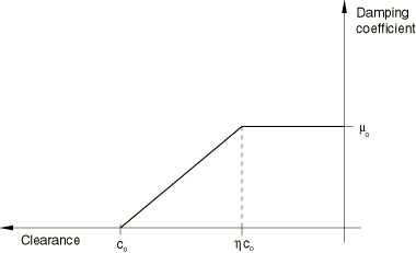
Figure 1: Contact Damping, damping coefficient

In Abaqus/Standard, this damping is mostly used to handle difficult problems like snap-through buckling or unstable contact. It doesn’t represent a real physical behavior; it’s a tool to help you get a solution when the model becomes unstable.

In Abaqus/Explicit, damping is more common. In fact, Abaqus contact damping is included by default in many cases, especially when you use softened contact or penalty contact. It helps reduce small vibrations or noise in the results. However, damping isn’t a magic fix. If overused, it can make your results less realistic. That’s why it’s important to understand how and when to apply it.

In the next section, we’ll compare how damping works in the two main solvers: Standard and Explicit.

1.1. Why is Abaqus Contact Damping important?

Contact damping is crucial in ensuring the stability and convergence of contact simulations. During these simulations, especially those involving large relative displacements, high strain rates, or significant material nonlinearities, the contact forces can change rapidly. These rapid changes can lead to numerical instabilities or oscillations, which affect the accuracy and convergence of the analysis.

By applying contact damping, Abaqus dissipates energy from the system, thereby reducing the likelihood of unstable or oscillatory contact forces. This stabilization is essential for maintaining the integrity and reliability of the simulation results.

1.2. When we need Abaqus Contact Damping?

Abaqus Contact damping is particularly useful in the following scenarios:

• Problems with large amounts of friction
• Post-buckling analyses
• Simulations involving large deformations
• Cases with material softening
• Multi-step analyses with significant changes in model stiffness
• Convergence issues: When sudden changes in contact constraints lead to convergence problems, such as in buckling problems involving contact.
• Softened or penalty contact: In Abaqus/Explicit, it helps dampen oscillations in these types of contact formulations.
• High-frequency oscillations: When rapid changes in contact forces cause numerical instabilities or oscillations that affect the accuracy of the analysis.

2. Application in Abaqus/Standard vs. Abaqus/Explicit

Both Abaqus/Standard and Abaqus/Explicit support contact damping, but they use it in different ways and for different reasons. Understanding how each solver handles it will help you apply it correctly and avoid misleading results.

• Abaqus/Standard: In Abaqus/Standard, contact damping is not used by default. It’s mainly intended as a numerical tool; a way to help the solver get through difficult steps when contact suddenly changes or when convergence issues appear. For example, if a model has snap-through behavior or buckling under contact constraints, Abaqus contact damping can smooth out the solution process. However, it should be used carefully. Since it adds artificial energy to the system, it can affect accuracy if applied too heavily. Think of it as a backup tool, not something to rely on for every contact problem.
• Abaqus/Explicit: Abaqus/Explicit uses contact damping more naturally. By default, a small amount of damping is already applied when using penalty contact or softened contact. This built-in damping, usually set to a critical damping fraction of 0.03, helps reduce high-frequency oscillations that don’t reflect real physics. These oscillations often appear when contact conditions change quickly, especially in dynamic simulations. This makes Abaqus contact damping a regular part of Explicit workflows, not just a troubleshooting tool.

It’s also worth noting how damping works in different directions. In both solvers, damping can be applied in the normal and tangential directions. In Abaqus/Standard, tangential damping is based on the relative sliding velocity.

In Abaqus/Explicit, it depends on the elastic slip rate, which is linked to friction behavior. That means in Explicit, tangential damping doesn’t resist full sliding, it only dampens small elastic slips. This is an important detail because it shows that damping behaves differently in Explicit when sliding is involved.

To sum up, use contact damping in Abaqus/Standard only when necessary, and tune it carefully. In Abaqus/Explicit, feel free to use it more freely, especially for noisy simulations. Still, remember that even in Explicit, too much damping can mask real behavior — so moderation is key.

3. How to Apply Contact Damping in Abaqus?

Contact damping in Abaqus is applied in both ABAQUS/Standard and ABAQUS/Explicit. The damping coefficient, which can be specified as a proportionality constant with units of pressure divided by velocity or as a unitless fraction of critical damping, defines the viscous damping force.

• ABAQUS/Standard: The damping coefficient is applied independent of the open/close state of the contact.
• ABAQUS/Explicit: The damping coefficient is applied only when the surfaces are in contact.

You can define Abaqus contact damping using either the CAE interface or keyword input. Both methods let you control how much damping to apply and in which direction.

3.1. Using the Abaqus CAE Interface

In Abaqus GUI, you can define contact damping inside a surface interaction property. To apply Abaqus contact damping in the CAE interface, start by opening the Interaction module. Then, either create a new interaction property or select an existing one to edit. Inside the dialog box that opens, go to the Mechanical section. From there, choose the Damping option. This is where you’ll define how the damping behaves during contact.

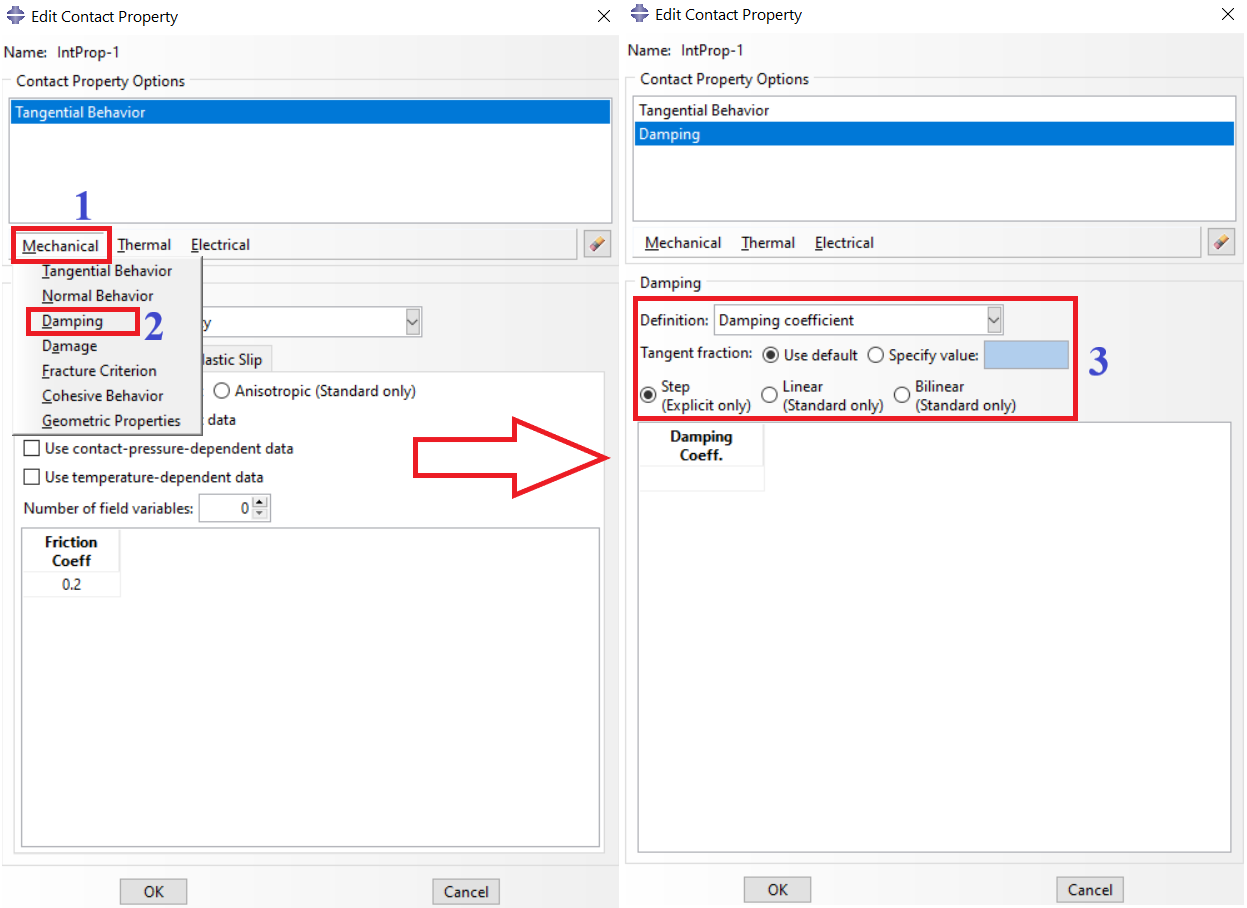
Figure 2: Applying Abaqus contact damping through Abaqus/CAE (GUI)

At this point, you have two main options:

• Damping Coefficient: In Abaqus/Standard, damping is often added to help with convergence. But if the damping is too high, it can change the results and hide real physical responses. So, the goal is to use just enough damping to stabilize the solution, but not so much that it distorts it.

A good starting point is to estimate the maximum relative velocity between contacting surfaces and the peak contact pressure in the model. You can do this by running the simulation without damping and observing the results. If the simulation fails, check the .msg file.

Abaqus reports the maximum nodal displacement increment at each time step. Divide that displacement by the time increment to get an approximate velocity. Then, estimate the damping coefficient using this:

Damping Coefficient ≈ Contact Pressure /Relative Velocity

This will give you a value that produces enough resistance to motion, but not so much that it overpowers real physical forces. You can try this value first, then reduce it gradually until the model becomes unstable again, and then go back one step.

• Critical Damping Fraction: You define it as a fraction of critical damping. This option is available only in Abaqus/Explicit. In Abaqus/Explicit, you can define damping as a fraction of critical damping. This option is unitless and easy to use. A typical value is 0.03, which is also the default in softened or penalty contact. It means 3% of the maximum damping that can be applied without causing instability.

Critical damping is simple and works well in most dynamic problems. However, it offers less control than a damping coefficient, especially if you need to tune damping based on contact pressure or velocity.

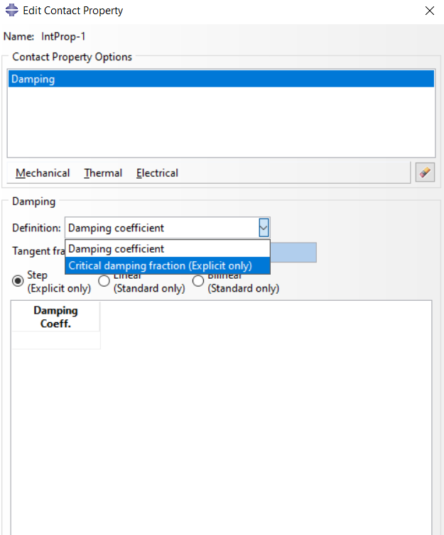
Figure 3: Damping coefficient and Critical damping fraction options

In Abaqus, damping can be defined using a step, linear, or bilinear function based on the clearance between contact surfaces (see figure 2).

• Step: In Abaqus/Explicit, you can also define the damping coefficient as a step-based value. This means the damping remains constant during a step, but you can assign a different value if needed in a new analysis step. However, this must be done manually by redefining or reassigning the interaction property. This option is useful when one step of your simulation (like an impact event) needs stronger damping than others.
• Linear: Damping decreases linearly from a maximum value at zero clearance to zero at a user-defined distance.
• Bilinear: Damping stays constant over an initial gap, then drops linearly to zero. This gives more control, especially when you expect small surface separations or bounces.

When you define Abaqus contact damping, you can apply it in the normal direction, the tangential direction, or both. But how these two work and when they apply depends on the solver you are using.

• Normal Damping: Normal damping resists motion perpendicular to the contact surface. It’s the most commonly used type. In both Abaqus/Standard and Abaqus/Explicit, normal damping adds a force that slows down surfaces as they come together or separate. This is helpful when dealing with contact bounces, convergence problems, or fast-changing contact states. To use normal damping, we must Tangent fraction on the Use Default
• Tangential Damping: Tangential damping resists motion along the contact surface, and slows down sliding. It’s optional and must be used together with normal damping. In Abaqus/Explicit tangential damping is active if The Tangent fraction is set on specify option and the value is specified.

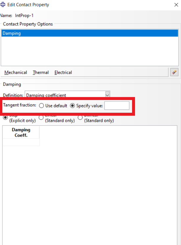
Figure 4: defining tangential damping in the interaction module

Remember to start with small damping values and increase gradually as needed. Excessive damping can lead to non-physical behavior or convergence issues.

3.2. Using Keyword Input

To apply contact damping through the input file, just look at the figure below and use the command “*Contact Damping”.

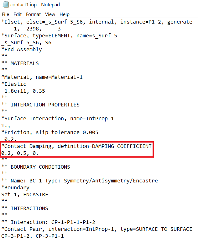
Figure 5: Abaqus Contact damping through the input file.

In the above figure, the damping is set to the damping coefficient type, and for the tangent fraction, the default option is selected. The first number represents the damping coefficient and the second and third numbers are the clearance values.

There is another damping called material damping. This one simulates how real materials internally resist motion and lose energy. It includes common methods like Rayleigh damping, modal damping, and viscoelastic damping. you can learn more about it in our blog: “Abaqus material damping“.

4. Abaqus Contact Stabilization VS Contact Damping

When solving contact problems in Abaqus, you might come across two different tools: Abaqus contact damping and Abaqus contact stabilization. At first, they may seem similar both help with convergence and simulation stability. But in reality, they work very differently and are meant for different situations.

• Contact Damping

Contact damping adds a viscous resistance based on how fast the two surfaces are moving relative to each other. It works just like a shock absorber: the faster things move, the more resistance it applies.

This is useful when:

• Contact changes suddenly (impact).
• You need to remove oscillations or bouncing.
• You want to stabilize motion during contact, not position.

• Contact Stabilization

Contact stabilization, on the other hand, is a broader method built into Abaqus/Standard. It adds artificial damping or stiffness to reduce rigid body motion or penetration when contact is newly forming. It’s controlled through contact controls, not surface interaction properties.

Use it when:

• Rigid surfaces move or drift before contact is engaged.
• You get errors about unconstrained motion.
• You want to suppress instability before contact happens.

As you can in the next figure, contact stabilization is available from the Interaction module, Contact Controls, and Stabilization tab.

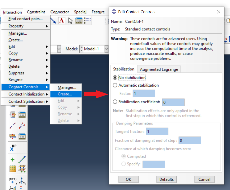
Figure 6: Contact Controls edit window

You’ll see three options:

• No stabilization: nothing added.
• Automatic stabilization: Abaqus chooses a damping coefficient for you. Despite being called “automatic,” the factor is not the damping coefficient itself, but rather a multiplier used internally by Abaqus to calculate the damping coefficient based on model data.
• Stabilization coefficient: you enter your own stabilization damping value. This value is used, without any further calculation or adjustment by Abaqus.

Both “automatic stabilization” and “stabilization coefficient” options apply damping only during the first step in which the contact control is active.

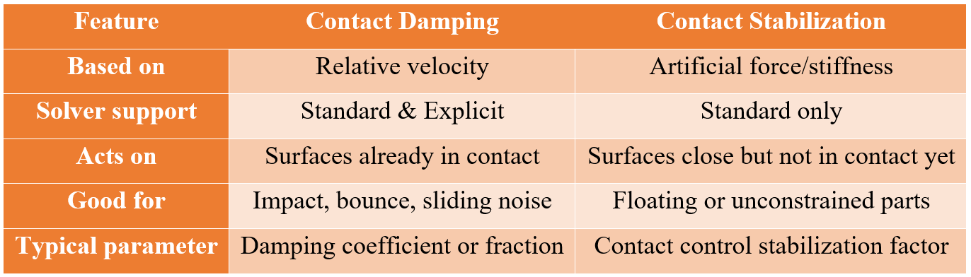
Figure 7: compare contact damping and contact stabilization

Note: Don’t confuse contact stabilization with automatic stabilization. Contact stabilization is applied only to contact pairs through contact controls and helps reduce rigid body motion during early contact. In contrast, automatic stabilization is applied to the entire model through step settings and is used to stabilize unstable static problems and large deformations.

They serve different purposes and should be used thoughtfully. If you want to know more about automatic stabilization, please follow our blog “Automatic Stabilization Abaqus of Unstable Problems | dissipated energy fraction, Damping factor”.

5. Conclusion

This article discussed contact damping in Abaqus, including what it is, how it functions, and how to apply it correctly in simulations. Contact damping is a numerical tool that helps manage instabilities during surface interactions like sliding or impact.

This topic is important because uncontrolled contact behaviors can cause convergence issues or produce noisy results. Proper use of damping improves simulation stability without distorting the physical meaning of the model.

The article first introduced the concept of contact damping, showing how it works like a shock absorber in simulations. Then it compared Abaqus/Standard and Abaqus/Explicit, explaining that damping is optional in Standard and automatic in many Explicit cases. Next, it covered implementation methods, including the CAE interface and keyword input options, with key formulas like the damping coefficient. It also differentiated contact damping from contact stabilization, showing they work in different stages of contact. Finally, it gave best practices to avoid errors like overusing damping or misusing stabilization.

In summary, we learned that contact damping is a helpful feature when applied carefully. Understanding its purpose, settings, and differences from stabilization ensures more stable and reliable Abaqus simulations.

Explore our comprehensive Abaqus tutorial page, featuring free PDF guides and detailed videos for all skill levels. Discover both free and premium packages, along with essential information to master Abaqus efficiently. Start your journey with our Abaqus tutorial now!