
Abaqus Plasticity: How to model plasticity in Abaqus?

Abaqus Plasticity provides advanced capabilities for modeling the plastic behavior of materials under various loading conditions. It offers a comprehensive suite of constitutive models, including isotropic, kinematic, and anisotropic plasticity models, to accurately capture the nonlinear and path-dependent behavior of solids undergoing plastic deformation.
Material plasticity is a fundamental property of materials that enables them to undergo permanent deformation without fracture when subjected to mechanical loads beyond their elastic limit. This phenomenon plays a crucial role in various engineering applications and is essential for understanding the behavior of materials under stress.
To model plasticity in Abaqus (Abaqus plasticity model), users must specify the appropriate plasticity model for the material. The model parameters can be calibrated using experimental data or empirical relationships. Once the plasticity model is defined, Abaqus uses advanced numerical methods to solve the governing equations and predict the plastic deformation of the material under various loading conditions.
In this article, we will discuss some of the plasticity theories and their application in Abaqus, and Hardening Plasticity laws to give you a better sight of modeling material plasticity. Let’s Start.
What is Plasticity Hardening in Abaqus? Is it isotropic hardening? or is it Johnson-cook hardening? What does even Hardening mean? All explained in the package below with 4 Practical examples which you can see them below. You can get all the files (subroutine, inp, etc) through this tutorial.
 |
|
1. Introduction of material plasticity
We often think of materials as having a simple, linear response to stress – apply pressure, they deform, release pressure, they return to their original shape. This is true for many materials within a specific range, but it only tells half the story. Beyond that limit, a fascinating phenomenon takes over: “Plasticity”.
Plasticity, in the context of materials science, describes the ability of a solid material to permanently deform under stress. Think of bending a paper clip. This permanent deformation is irreversible – the paper clip won’t spring back to its original shape.
Understanding material plasticity is crucial for numerous applications:
- Structural design
Architects and engineers rely on this knowledge to design structures that can withstand immense stress without permanent failure. Bridges, buildings, and even airplanes are engineered to harness the flexibility of materials while remaining stable under load.
- Manufacturing
Plasticity is the foundation of many manufacturing processes like forging and rolling, where metal is shaped by applying tremendous force.
- Material science research
Studying the mechanics of plasticity allows scientists to develop new materials with specific properties, such as enhanced strength and resilience. This leads to innovations in aerospace, medical implants, and various other fields.
2. Modeling of Uniaxial Behavior in Plasticity
In order to obtain a solution to a deformation problem, it is necessary to idealize the stress-strain behavior of the material. The following idealized models deserve note.
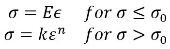
2.1. Elastic-perfectly plastic model
In some instances, it is permissible and convenient to neglect the effect of work hardening and assume that the plastic flow occurs as the stress has reached the yield stress ![]() . Thus, the uniaxial tension stress-strain relation may be expressed as:
. Thus, the uniaxial tension stress-strain relation may be expressed as:
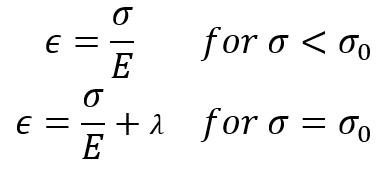
Where E is Young’s modulus, and ![]() is a scalar to be determined and is greater than 0.
is a scalar to be determined and is greater than 0.
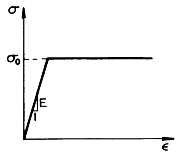
Figure 1: Elastic-perfectly plastic stress-strain curve [1]
 |
Hardening Plasticity tutorial package syllabus:
|
2.2. Elastic-linear work-hardening model
In the elastic-linear work-hardening model, the continuous curve is approximated by two straight lines, thus replacing the smooth transition curve with a sharp breaking point, the ordinate of which is taken to be the elastic limit stress or the yield strength ![]() . The first straight-line branch of the diagram has a slope of Young’s modulus, E. The second straight-line branch, representing in an idealized fashion the strain-hardening range, has a slope of
. The first straight-line branch of the diagram has a slope of Young’s modulus, E. The second straight-line branch, representing in an idealized fashion the strain-hardening range, has a slope of ![]() . The stress-strain relation for a monotonic loading in tension has the form:
. The stress-strain relation for a monotonic loading in tension has the form:
Figure 2: Elastic-linear work-hardening stress-strain curve [1]
 |
⭐⭐⭐ Free Abaqus Course | ⏰10 hours Video 👩🎓+1000 Students ♾️ Lifetime Access
✅ Module by Module Training ✅ Standard/Explicit Analyses Tutorial ✅ Subroutines (UMAT) Training … ✅ Python Scripting Lesson & Examples |
2.3. Elastic-exponential hardening model
Consider a power expression of the type:
where k and n are two characteristic constants of the material to be determined to best fit the experimentally obtained curve. If ![]() represents the total strain, the curve should pass through the point representing the yield stress and the corresponding elastic strain. The power expression should be used only in the strain-hardening range.
represents the total strain, the curve should pass through the point representing the yield stress and the corresponding elastic strain. The power expression should be used only in the strain-hardening range.
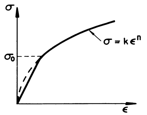
Figure 3: Elastic-exponential hardening stress-strain curve [1]
2.4. Ramberg-Osgood model
The nonlinear stress-strain curve as shown in figure 4 has the following expression:
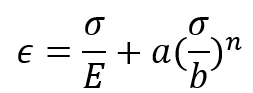
in which a, b, and n are material constants. The initial slope of the curve takes the value of Young’s modulus E at ![]() , and decreases monotonically with increasing loading. Since the model has three parameters, it allows for a better fit of real stress-strain curves.
, and decreases monotonically with increasing loading. Since the model has three parameters, it allows for a better fit of real stress-strain curves.
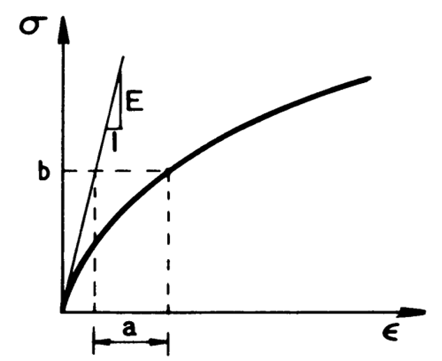
Figure 4: Ramberg-Osgood stress-strain curve [1]
3. Abaqus Plasticity model (Modeling)
Abaqus provides a comprehensive library of plasticity models that cover a wide range of material behaviors. These models are shown in Figure 5.
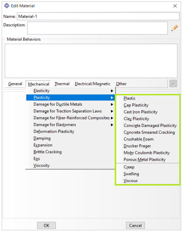
Figure 5: Abaqus plasticity models for different material behaviors
As you can see there are several options for modeling plasticity in Abaqus which are out of the scope of this discussion. In this post, we will introduce the first option which is ‘Plastic’, and uses Mises or Hill yield surfaces with associated plastic flow. It is one of the most common models you may use in your simulations.
Speaking of Yield surface; Do you know what exactly it is?? there is complete description of it in our tutorial video: “What is Yield Surface?“
3.1. Plastic Region Definition in Abaqus
In Abaqus/CAE to define this plasticity model you must do as following:
- Go to the “Property” module
- Define a Material
- Mechanical> Plasticity> Plastic
After that, you must provide some data that we will discuss about them here. These data are shown in figure 6.
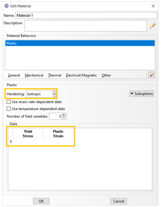
Figure 6: Data for plastic definition in Abaqus
You need to determine the hardening and enter the plastic region data including plastic strain and its corresponding yield stress in this window.
Let’s first determine how to enter the appropriate data for the plastic region.
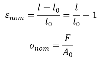
When defining plasticity data in Abaqus, you must use true stress and true strain. Abaqus requires these values to interpret the data in the input file correctly. However, quite often material test data are supplied using values of nominal stress and strain. In such situations, you must convert the plastic material data from nominal stress and strain to true stress and strain.
The relationship between true strain and nominal strain is as follows:
![]()
The relationship between true stress and nominal stress is formed by considering the incompressible nature of the plastic deformation and assuming the elastic volumetric deformation is negligible. So, the relationship between true stress and nominal stress and strain is:
You can Learn how to work with UHARD subroutine to define any Hardening you want with a very simple example: “Implementation of UHARD Subroutine for isotropic hardening (formulation based) in simple model“
![]()
Where in the previous relations, ![]() and
and ![]() can be expressed as:
can be expressed as:
The strains provided in material test data used to define the plastic behavior are not likely to be the plastic strains in the material. Instead, they will probably be the total strains in the material. You must decompose these total strain values into the elastic and plastic strain components. The plastic strain is obtained by subtracting the elastic strain, defined as the value of true stress divided by Young’s modulus, from the value of total strain (Figure 7). This relationship is written as:
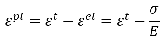
Where ![]() is true plastic strain,
is true plastic strain, ![]() is true total strain,
is true total strain, ![]() is true elastic strain,
is true elastic strain, ![]() is true stress, and E is Young’s modulus.
is true stress, and E is Young’s modulus.
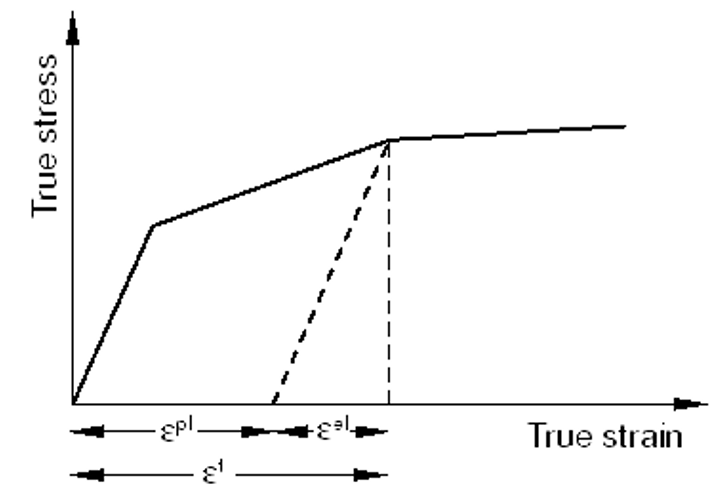
Figure 7: Strain components in a deformation
Abaqus connects your stress-strain data pairs with a series of straight-line segments to form a continuous, piecewise linear plasticity curve. You can use any number of data pairs to approximate the actual material behavior; therefore, it is possible to get a very close approximation of the actual material behavior.
Let’s implement the previous concepts in an example.
3.2. Example of converting material test data to Abaqus input
The stress-strain curve in figure 8 will be used as an example of how to convert the test data defining a material’s plastic behavior into the appropriate input format for Abaqus.
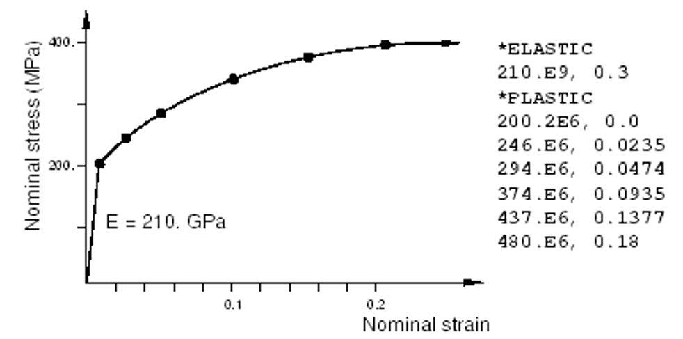
Figure 8: Elastic-plastic material behavior and corresponding Abaqus input data
The first step is to use the equations relating the true stress to the nominal stress and strain and the true strain to the nominal strain to convert the nominal stress and nominal strain to true stress and true strain. Once these values are known, the equation relating the plastic strain to the total and elastic strains which were shown earlier can be used to determine the plastic strains associated with each yield stress value. The converted data are shown in table 1.
Table 1: Converting nominal stress and strain to true stress and strain
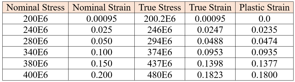
As you can see in figure 8, the ‘True Stress’ and ‘Plastic Strain’ columns of this table are entered as Abaqus input data for the plastic definition.
It’s good for you to obtain the values in table 1 from the nominal stress and strain as a practice using the mentioned relations.
3.3. Perfect Plasticity | Elastic perfectly plastic Abaqus
Perfect plasticity means that the yield stress does not change with plastic strain. It can be defined in tabular form for a range of temperatures and/or field variables; a single yield stress value per temperature and/or field variable specifies the onset of yield.
Imagine the only inelastic material data available for steel are its yield stress (380 MPa) and its strain at failure (0.15). You decide to assume that the steel is perfectly plastic: the material does not harden, and the stress can never exceed 380 MPa as in figure 10.
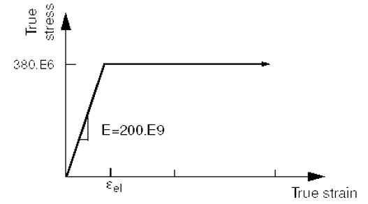
Figure 10: Stress-strain behavior for the perfectly plastic steel
The initial yield stress at zero plastic strain is 380 MPa. Since you are modeling the steel as perfectly plastic, no other yield stresses are required (Figure 11).
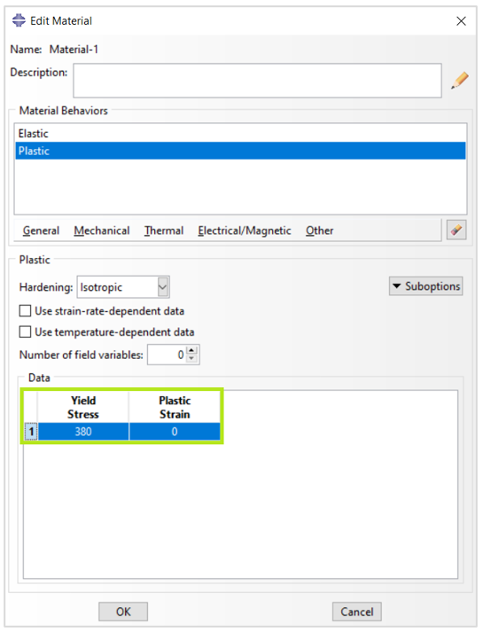
Figure 11: Define an elastic-perfectly plastic material
4. Hardening Plasticity in Abaqus
Now let’s see what are the different hardening plasticity types you can define in Abaqus plastic.
In Abaqus, a perfectly plastic material (with no hardening) can be defined, or work hardening can be specified. Isotropic hardening is available in both Abaqus/Standard and Abaqus/Explicit; Johnson-Cook hardening is available only in Abaqus/Explicit. In addition, Abaqus provides kinematic hardening for materials subjected to cyclic loading.
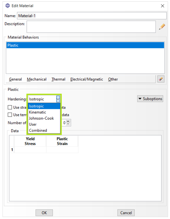
Figure 9: Different hardening plasticity types for Abaqus plasticity
4.1. Isotropic Hardening Abaqus
For a perfectly plastic material, the equation for the fixed yield surface has the form, ![]() , where k is a constant. The simplest work-hardening rule is based on the assumption that the initial yield surface expands uniformly without distortion and translation as plastic flow occurs, as shown schematically in figure 12. The size of the yield surface is now governed by the value
, where k is a constant. The simplest work-hardening rule is based on the assumption that the initial yield surface expands uniformly without distortion and translation as plastic flow occurs, as shown schematically in figure 12. The size of the yield surface is now governed by the value ![]() , which depends upon plastic strain history.
, which depends upon plastic strain history.
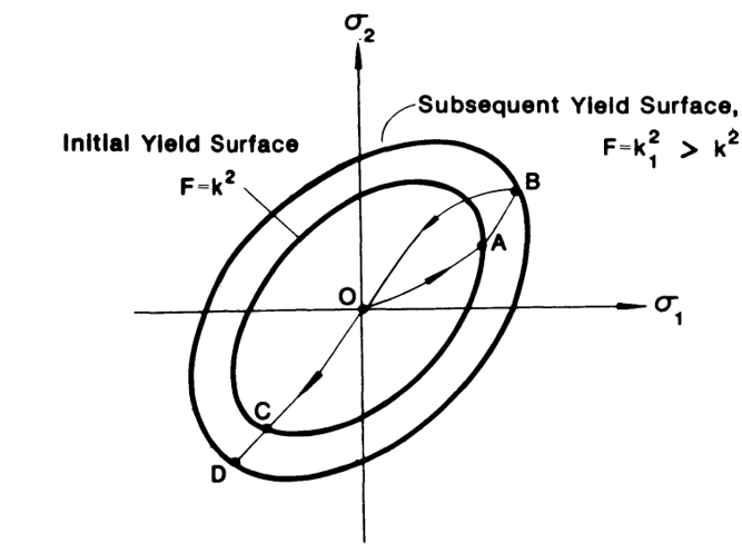
Figure 12: Subsequent yield surface for isotropic-hardening material [1]
The isotropic hardening Abaqus plasticity model is simple to use, but it applies mainly to monotonic loading without stress reversals. So, it cannot account for the Bauschinger effect exhibited by most structural materials.
If isotropic hardening is defined, the yield stress, ![]() , can be given as a tabular function of plastic strain and, if required, of temperature and/or other predefined field variables. The yield stress at a given state is simply interpolated from this table of data, and it remains constant for plastic strains exceeding the last value given as tabular data.
, can be given as a tabular function of plastic strain and, if required, of temperature and/or other predefined field variables. The yield stress at a given state is simply interpolated from this table of data, and it remains constant for plastic strains exceeding the last value given as tabular data.
|
Hardening Plasticity tutorial package syllabus:
|
4.2. Kinematic Hardening Abaqus
The kinematic hardening Abaqus plasticity rule assumes that during plastic deformation, the loading surface translates as a rigid body in stress space, maintaining the size, shape, and orientation of the initial yield surface (Figure 13).
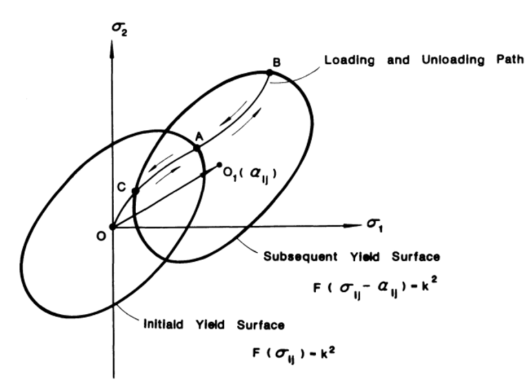
Figure 13: Subsequent yield surface for kinematic-hardening material [1]
As a consequence of assuming a rigid-body translation of the loading surface, the kinematic hardening rule predicts an ideal Bauschinger effect for a complete reversal of loading conditions.
Two kinematic hardening models are provided in Abaqus to model the cyclic loading of metals. The linear kinematic model approximates the hardening behavior with a constant rate of hardening. The more general nonlinear isotropic/kinematic model will give better predictions but requires more detailed calibration.
To specify the nonlinear combined isotropic/kinematic model, you must select the ‘Combined’ hardening.
Bauschinger effect and kinematic hardening. You can learn them in practice with this example and plus how to use VUMAT subroutine for Hardening: “Writing VUMAT Subroutine for Kinematic Hardening Plasticity“
4.3. Combined Isotropic and Kinematic Hardening in Abaqus
In isotropic hardening Abaqus and kinematic hardening Abaqus models, different features of the behavior of materials under different loadings, such as cyclic or combined loadings, are investigated. The combined isotropic and kinematic hardening model allows you to model both types of hardening simultaneously in a single simulation. This model is beneficial when materials are subjected to complex loadings or reversible conditions in compression and tension.
In Abaqus, the combined isotropic and kinematic hardening model can be implemented using both built-in material options and user-defined subroutines. For many standard applications, Abaqus provides integrated features that allow users to specify the parameters for both hardening mechanisms directly, streamlining the setup for complex loading conditions. However, when simulations require more tailored or advanced hardening behavior—particularly under non-standard or highly cyclic loadings—a user subroutine (such as UMAT or VUMAT) offers the flexibility to define the material response in greater detail.
In this section, we focus on its application via subroutines, highlighting how this approach enables precise control over the hardening behavior in scenarios where reversible conditions in compression and tension demand an accurate representation of both isotropic expansion and directional yield surface translation.
4.3.1. Definition and Usage of the Combined Hardening Model
In many engineering simulations, such as cyclic or dynamic analyses, the material is subjected to loadings that involve both a change in the size of the yield surface (associated with isotropic hardening) and a displacement in its position (associated with kinematic hardening). These two processes co-occur in practice, and if only one of them is considered, the results may differ significantly from reality.
A typical example of this condition is the phenomenon of ratcheting. In ratcheting, when a body is subjected to cyclic loading (i.e., the load is applied intermittently), plastic deformation in a given direction accumulates continuously over time, even if it is intermittent and without change in the periodicity. In this case, in addition to the increase in the yield surface (due to isotropic hardening), the yield surface also shifts (a result of kinematic hardening). This behavior is critical in materials under dynamic or cyclic loading that causes a permanent change in the yield surface.
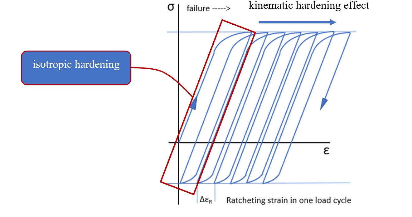
Figure 14: Effects of kinematic and isotropic hardening on ratcheting phenomenon
In the combined model, we look at two kinds of hardening—isotropic and kinematic. This lets us see how both sides change and helps us fully simulate the behavior. Basically, the combined model merges these two effects into one equation or algorithm. This combination is typically modeled as follows:
![]()
 are the stresses and forces acting on the material.
 is the position of the yield surface that changes under the influence of kinematic hardening.
 is the plastic strain that indicates the rate of change in isotropic hardening.
 is the initial yield stress that indicates the moment the material enters the plastic region.
In this model, at each moment of the simulation, the isotropic and kinematic combinations will be as follows:
In this equation:
 is the plastic strain, which indicates the rate of change in the yield surface.
 is the isotropic hardening coefficient, which indicates the rate of increase in the size of the yield surface.
 is the kinematic hardening coefficient, which indicates the rate of displacement of the yield surface.
In this way, this model allows us to predict the behavior of materials more accurately and realistically.
4.3.2. Applications of the Combined Model in Complex Simulations
The combined isotropic and kinematic hardening model is widely used in complex simulations due to its ability to capture material behavior accurately under intricate loading conditions. This model is particularly beneficial in scenarios where the material experiences simultaneous changes in the yield surface’s size and location.
As mentioned earlier, one of the most significant phenomena that the combined hardening model can simulate is ratcheting, where the material undergoes permanent plastic deformation even under cyclic loading. Other applications of this hardening model include:
- Metal Forming Simulations
In metal forming processes like rolling, extrusion, or casting, materials change shape significantly. The combined hardening model helps track how the yield surface shifts under stress and strain. This model is useful for high plastic strain and large deformations, allowing CAE users to design better processes, avoid defects, and improve the final product.
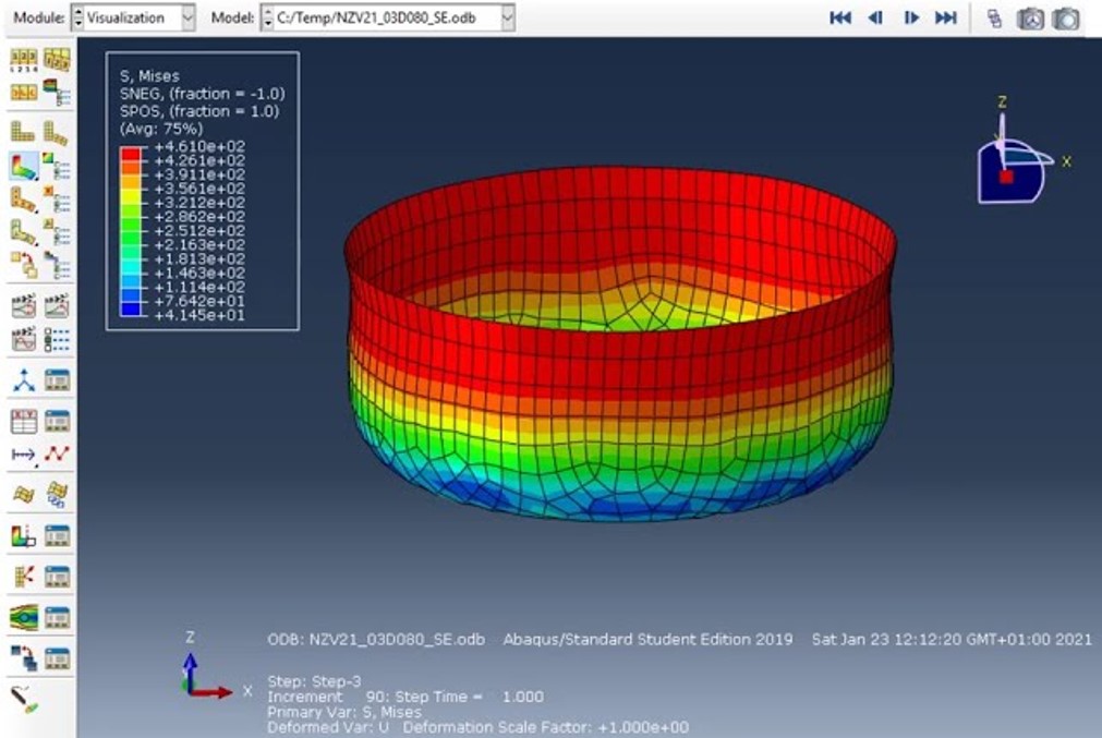
Figure 15: Effects of kinematic and isotropic hardening on Metal Forming Simulations
In metal forming, the use of both isotropic and kinematic hardening is critical because the material undergoes complex, multi-directional deformations. The isotropic component accounts for the uniform increase in yield stress as plastic deformation accumulates, representing an overall strengthening of the material. Meanwhile, the kinematic component specifically captures the translation of the yield surface in stress space, which is essential for modeling phenomena like the Bauschinger effect—commonly observed during load reversals in forming operations. This dual approach ensures that both the global hardening due to overall plasticity and the directional shifts in yielding due to localized strain paths are accurately represented.
- Nonlinear and Dynamic Analysis
In nonlinear and dynamic analyses, like those with explosions or impacts, materials can behave in complex ways. As they deform and harden, the yield surface changes in size and position. The combined isotropic and kinematic hardening model is great for capturing these responses under dynamic loads.
The material’s reaction depends on the applied stress and accumulated plastic strain, which influence the yield surface. This model offers a clearer view of material behavior in extreme conditions, making it ideal for blast analysis, impact simulations, and crash tests.
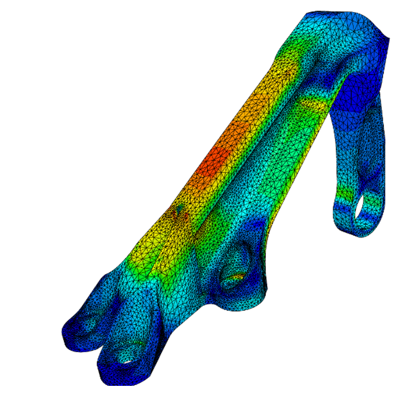
Figure 16: Nonlinear and Dynamic Analysis using the kinematic and isotropic hardening [Ref]
During dynamic events, such as impacts or explosions, the loading conditions change rapidly and non-uniformly. The isotropic hardening aspect models the overall increase in resistance due to cumulative plastic deformation, which is crucial when the material is uniformly strained over a short period. In contrast, the kinematic hardening component is essential for capturing the directional movement of the yield surface as the loading path shifts abruptly. This is particularly important for accurately predicting material response under cyclic or transient loads where directional effects, such as stress reversals, can influence the subsequent yielding behavior.
- Damage and Fracture Simulations
In damage and fracture simulations, figuring out how materials break down under stress is key for building safe and reliable structures. When materials go through repeated loads, using a combined isotropic and kinematic hardening model helps track the movement of the yield surface and when plastic deformation starts, which is crucial for understanding material damage. For more information on this, see Abaqus crack and fracture mechanics.
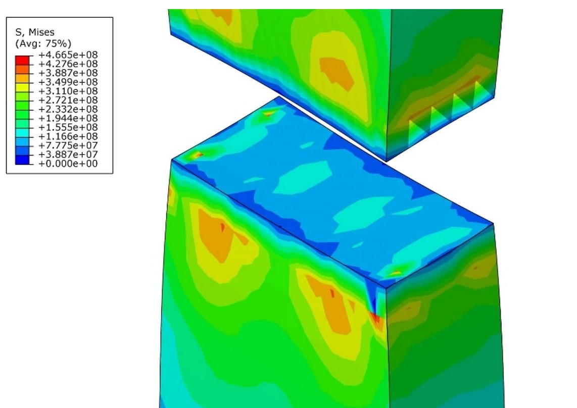
Figure 17: Using kinematic and isotropic hardening to simulate damage in Abaqus
In the context of damage and fracture simulations, incorporating both hardening mechanisms provides a more nuanced view of material degradation.
The isotropic hardening component reflects the overall increase in yield stress due to cumulative plastic deformation, which is important for assessing the material’s capacity to withstand continuous loading. Conversely, the kinematic hardening element captures localized shifts in the yield surface that can lead to stress concentrations and eventual crack initiation.
This separation of effects allows engineers to distinguish between general strengthening and localized softening or directional shifts that precipitate failure, leading to more accurate predictions of fracture initiation and growth.
4.4. Johnson-Cook Isotropic Hardening
Johnson-Cook hardening plasticity is a particular type of isotropic hardening in Abaqus/Explicit where the yield stress is given as an analytical function of equivalent plastic strain, strain rate, and temperature. This hardening law is suited for modeling the high-rate deformation of many materials including most metals.
For detailed information about Johnson-Cook hardening, we recommend to see the following link:
Introduction to Abaqus Johnson-Cook Model: Accurately Model High-Strain rate Events
4.5. User Hardening
In Abaqus/Standard the yield stress for isotropic hardening, ![]() , can alternatively be described through the user subroutine UHARD.
, can alternatively be described through the user subroutine UHARD.
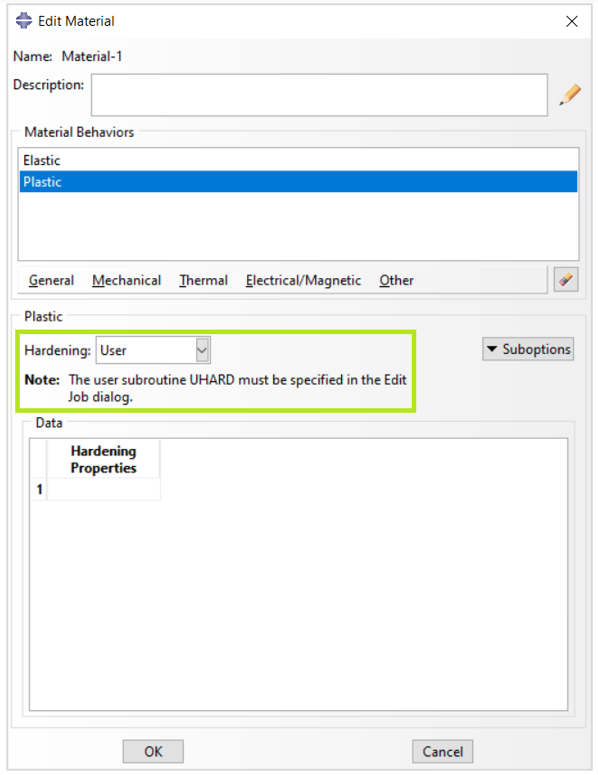
Figure 18: Defining User hardening in Abaqus plasticity
For detailed information about UHARD subroutine, we recommend to see the following link:
UHARD Subroutine (VUHARD Subroutine) in ABAQUS
we’ll dive into the VUMAT and UHARD subroutines in Abaqus, which are used to simulate plastic behavior with kinematic and isotropic hardening. These subroutines are implemented using FORTRAN code and are essential for modeling changes in stress and plastic strain in advanced simulations. We’ll walk you through how to use these subroutines and share the corresponding code in detail.
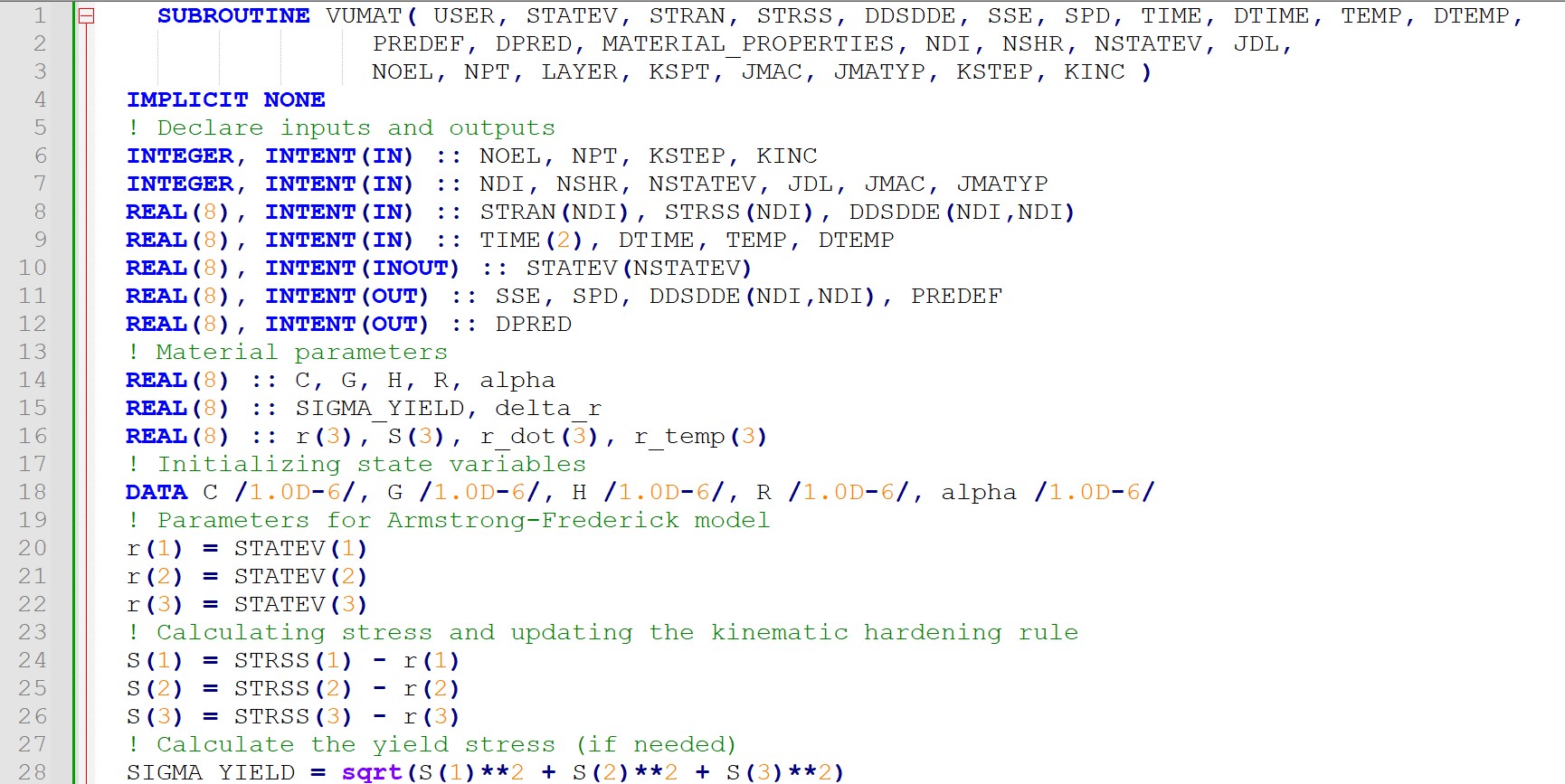
4.5.1. VUMAT Subroutine for Kinematic Hardening
In Start Writing Your 1st UMAT Abaqus & VUMAT Abaqus article, we fully explained the VUMAT subroutine. In this blog, we intend to explain the developed relations for kinematic hardening with a practical example. So, what are you waiting for? Let’s get started.
A classical kinematic hardening model, such as the Armstrong-Frederick or Prager model, in which the yield surface changes randomly and incrementally, can be simulated in Abaqus. Here, we examine how a simple Armstrong-Frederick model for kinematic hardening works. In this model, the stiffness update is applied in the direction of plastic strain, and the yield surface changes automatically according to the strain history. The Armstrong-Frederick model is typically expressed as follows:
![]()
Where:
- r is the kinematic stiffness vector (which is typically changed to model yield surfaces).
- S are the equivalent stresses.
- c is the matrix of model coefficients.
 is the rate of change of stiffness.
To implement this model in Abaqus in Fortran and as a VUMAT (subroutine for defining a behavioral model), a number of input parameters must be considered, including the stress-strain history and model parameters (such as 𝑐 and 𝑟).
 |
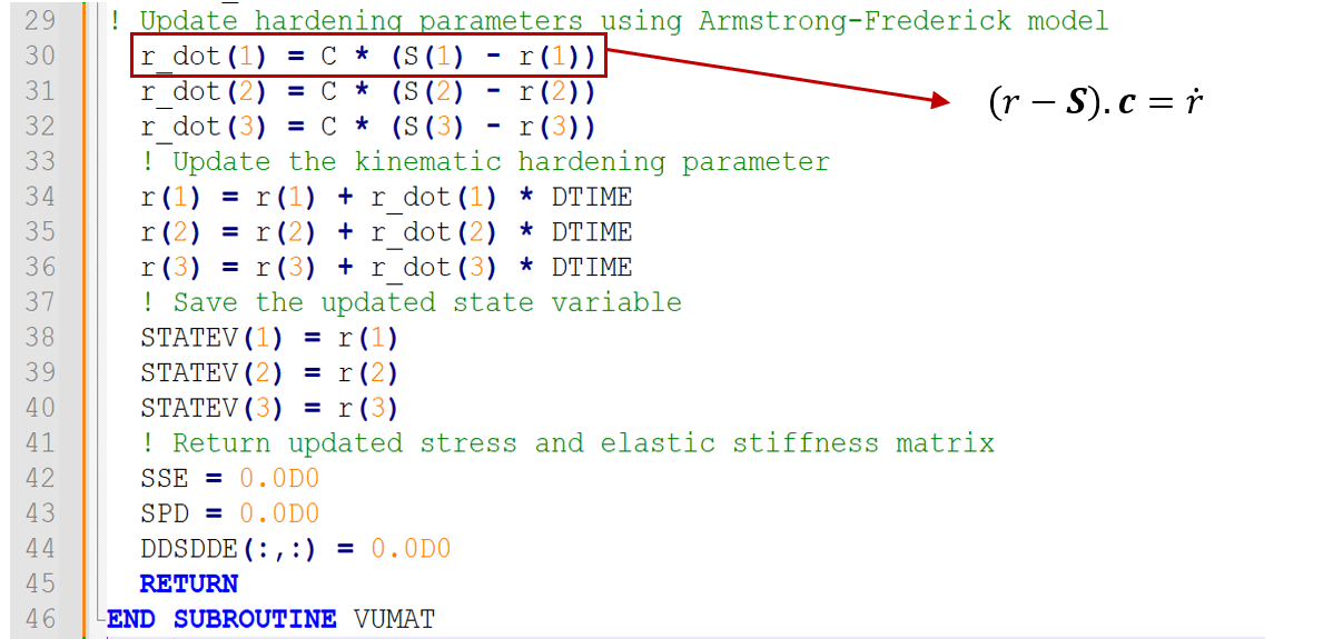 |
VUMAT subroutine for kinematic hardening
In this code, the necessary inputs including stresses, strains, and material parameters are first defined. Kinematic model parameters such as r, S, ![]() , and various model coefficients (such as C, G, H, and R) are also defined.
, and various model coefficients (such as C, G, H, and R) are also defined.
Calculation of equivalent stresses: In this section, the difference between equivalent stresses and hardness changes along the hardening history is calculated.
Updating the hardening parameters: Using the Armstrong-Frederick relations, the hardening parameters 𝑟 are updated according to the rate of change.
Maintain material history: Updated values for 𝑟 are stored in the STATEV variable to be used in later stages of the analysis.
Calculation of the strength matrix: In this code, the plastic strength matrix (DDSDDE) is assumed to be zero by default, which can be calculated according to specific models if needed.
4.5.2. UHARD Subroutine for Isotropic Hardening
The UHARD subroutine in Abaqus defines plastic behavior with isotropic hardening. This behavior means the material increases its stiffness and resistance to deformation (yield stress) without changing in different directions during load application. This subroutine is commonly used in plastic models, where the behavior of the material changes uniformly in all directions when more load is applied.
This subroutine is based on classical models for isotropic hardening, which connect changes in yield stress to plastic strain. Basically, the yield stress (Sy) changes are typically described as:
![]()
Where in this equation:
 is the current yield stress.
 is the initial yield stress.
- H is the isotropic hardness.
 is the plastic strain.
In this example, we use FORTRAN code to define isotropic hardening. This code introduces a FORTRAN subroutine into Abaqus to simulate plastic behavior with isotropic hardening.
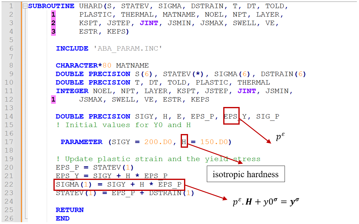
UHARD subroutine for isotropic hardening
Input and output parameters:
- S: Current stresses.
- STATEV: Internal states (such as plastic strain and stiffness state).
- SIGMA: Yield stress.
- DSTRAIN: Entered plastic strain.
- T, DT, TOLD: Time and times related to the analysis.
- MATNAME: Material name.
Other parameters are related to the state and numerical details of the model.
Definition of initial parameters:
SIGY and H are the initial yield stress and isotropic hardness, respectively. Here, SIGY = 200 MPa and H = 150 MPa are assumed to be constant.
Calculation of ultimate yield stress:
Using the relation ![]() , the new yield stress is obtained.
, the new yield stress is obtained.
Here, SIGMA(1) is updated to reflect the new values of the yield stress.
Updating the plastic strain:
The plastic strain STATEV(1) is also updated to reflect the changes in plastic strain after each analysis step.
What an amazing way we came through! Time to summarize what we have learned in this way.
5. Summary
We started our discussion by clarifying the importance of plasticity subject. Then we introduced some of the common plastic behaviors in materials. In advance, we talked about Abaqus plasticity and some of the capabilities of Abaqus to model plasticity.
In Abaqus, plasticity is implemented using a variety of material models, each of which is tailored to capture the specific behavior of a particular material or class of materials.
An important aspect of Abaqus plasticity is the use of hardening plasticity laws to describe the evolution of the material’s yield stress with plastic strain. Abaqus provides several built-in hardening laws, including isotropic, kinematic, and mixed hardening, as well as the ability to define user-defined hardening laws.
In the end, we appreciate for reading this article. Don’t forget to leave us your comments about this article to improve our content quality. Wish you the Best.
Now that you have understand what Hardening is and the types of hardening in Abaqus, don’t you want to learn them in action?? 4 Practical examples which you can see them below. You can get all the files (subroutine, inp, etc) through this tutorial.
|
|
Explore our comprehensive Abaqus tutorial page, featuring free PDF guides and detailed videos for all skill levels. Discover both free and premium packages, along with essential information to master Abaqus efficiently. Start your journey with our Abaqus tutorial now!
6. Users ask these questions
Defining the plastic properties is a common thing in Abaqus and so there are a lot of questions regarding this matter in many platforms and social media; therefore, we decided to answer a few of them.
I. Plastic region
Q: Having a perfect plastic region doesn’t make any convergence issues?
A: To avoid convergence problems, add a slight slope in the perfect plastic region. You can add a perfect plastic region like in figure 1. But you may encounter a convergence issue because the plastic strain is increasing in this model while the stress remains at the same value. Therefore, add a slight slope to avoid this issue (see figure 2). Note that all values in figures are just for example and don’t have to be true.
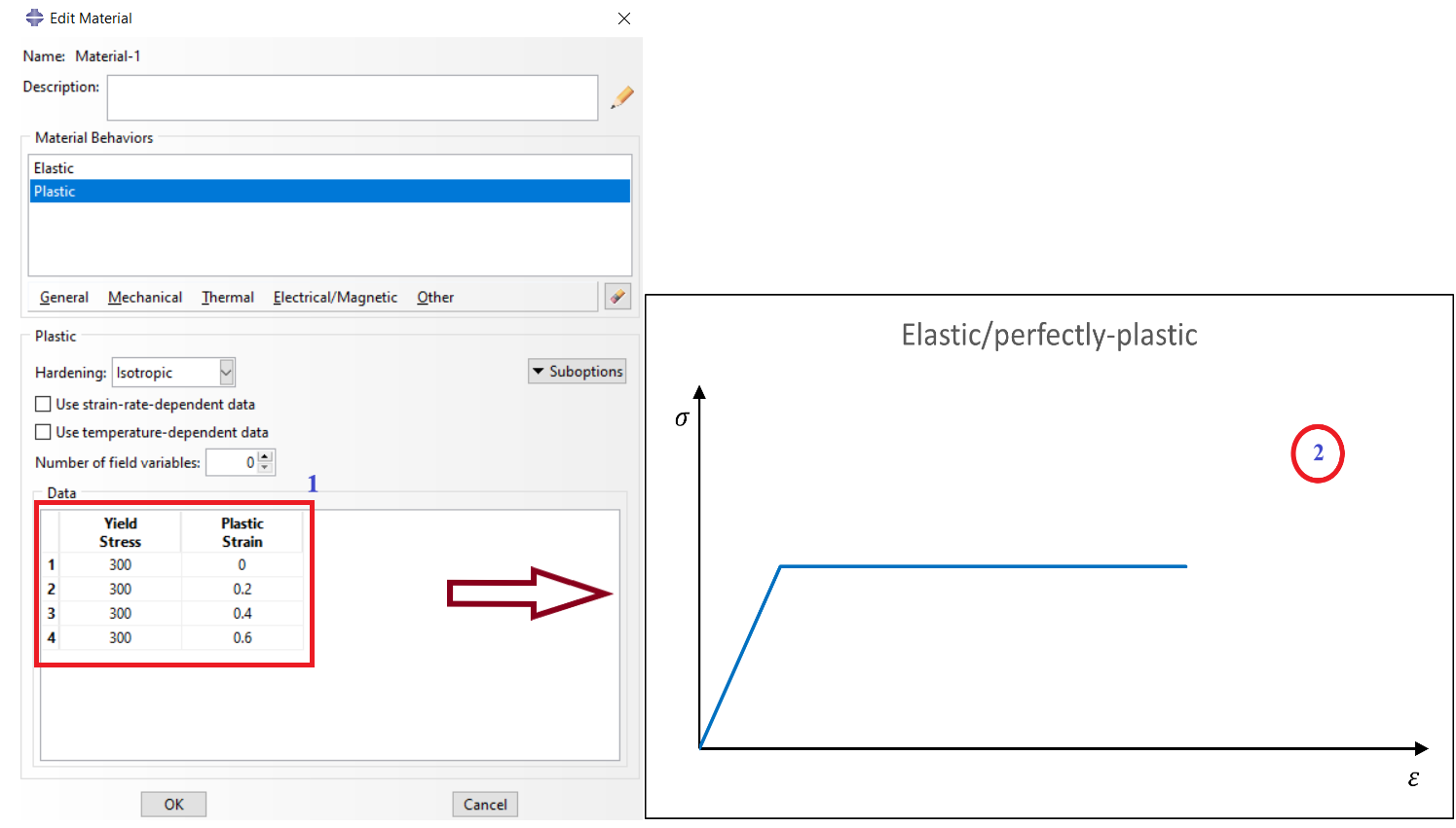
Figure 1: Perfect plastic region
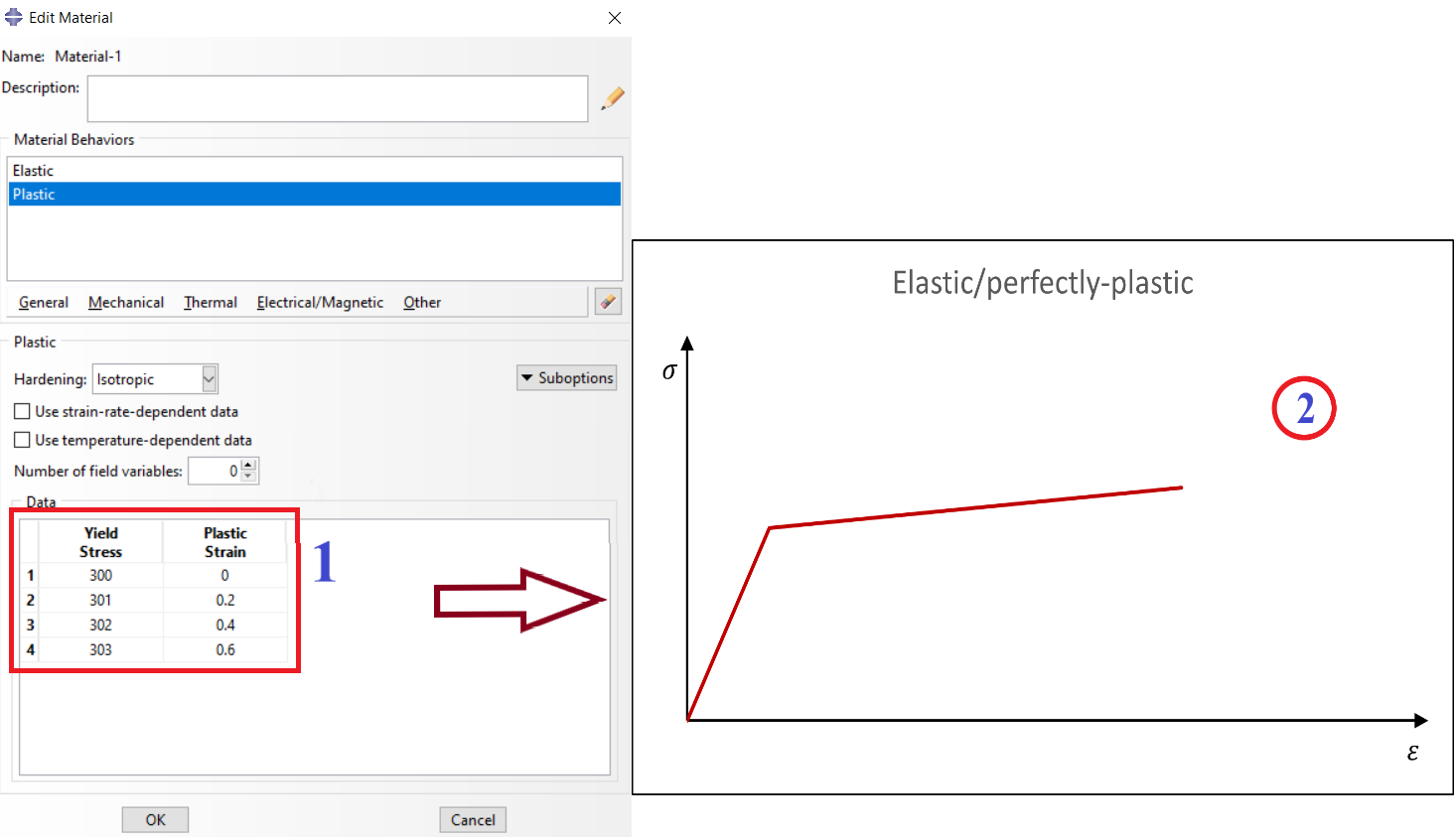
Figure 2: Perfect plastic region with slight slope