

Abaqus Plasticity provides advanced capabilities for modeling the plastic behavior of materials under various loading conditions. It offers a comprehensive suite of constitutive models, including isotropic, kinematic, and anisotropic plasticity models, to accurately capture the nonlinear and path-dependent behavior of solids undergoing plastic deformation.
Material plasticity is a fundamental property of materials that enables them to undergo permanent deformation without fracture when subjected to mechanical loads beyond their elastic limit. This phenomenon plays a crucial role in various engineering applications and is essential for understanding the behavior of materials under stress.
To model plasticity in Abaqus (Abaqus plasticity model), users must specify the appropriate plasticity model for the material. The model parameters can be calibrated using experimental data or empirical relationships. Once the plasticity model is defined, Abaqus uses advanced numerical methods to solve the governing equations and predict the plastic deformation of the material under various loading conditions.
In this article, we will discuss some of the plasticity theories and their application in Abaqus to give you a better sight of modeling material plasticity. Let’s Start.
1. Introduction of material plasticity
We often think of materials as having a simple, linear response to stress – apply pressure, they deform, release pressure, they return to their original shape. This is true for many materials within a specific range, but it only tells half the story. Beyond that limit, a fascinating phenomenon takes over: “Plasticity”.
Plasticity, in the context of materials science, describes the ability of a solid material to permanently deform under stress. Think of bending a paper clip. This permanent deformation is irreversible – the paper clip won’t spring back to its original shape.
Understanding material plasticity is crucial for numerous applications:
- Structural design
Architects and engineers rely on this knowledge to design structures that can withstand immense stress without permanent failure. Bridges, buildings, and even airplanes are engineered to harness the flexibility of materials while remaining stable under load.
- Manufacturing
Plasticity is the foundation of many manufacturing processes like forging and rolling, where metal is shaped by applying tremendous force.
- Material science research
Studying the mechanics of plasticity allows scientists to develop new materials with specific properties, such as enhanced strength and resilience. This leads to innovations in aerospace, medical implants, and various other fields.
1.1. Modeling of Uniaxial Behavior in Plasticity
In order to obtain a solution to a deformation problem, it is necessary to idealize the stress-strain behavior of the material. The following idealized models deserve note.
1.1.1. Elastic-perfectly plastic model
In some instances, it is permissible and convenient to neglect the effect of work hardening and assume that the plastic flow occurs as the stress has reached the yield stress ![]() . Thus, the uniaxial tension stress-strain relation may be expressed as:
. Thus, the uniaxial tension stress-strain relation may be expressed as:
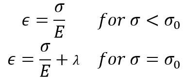
Where E is Young’s modulus, and ![]() is a scalar to be determined and is greater than 0.
is a scalar to be determined and is greater than 0.
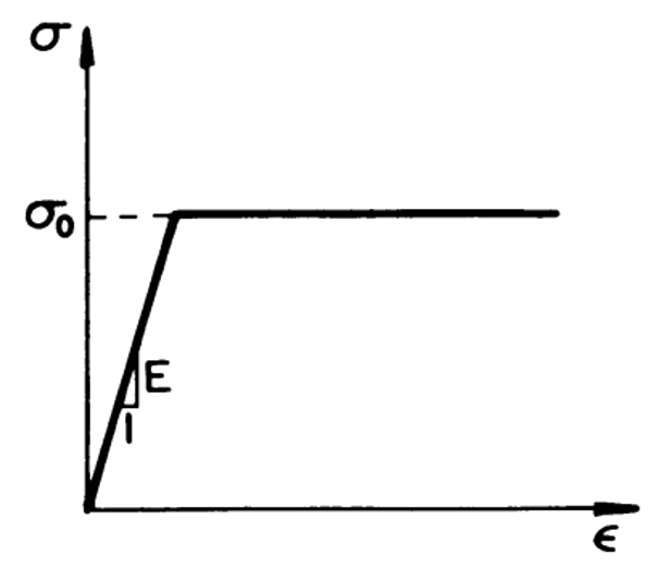
Figure 1: Elastic-perfectly plastic stress-strain curve [1]
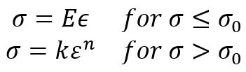
1.1.2. Elastic-linear work-hardening model
In the elastic-linear work-hardening model, the continuous curve is approximated by two straight lines, thus replacing the smooth transition curve with a sharp breaking point, the ordinate of which is taken to be the elastic limit stress or the yield strength ![]() . The first straight-line branch of the diagram has a slope of Young’s modulus, E. The second straight-line branch, representing in an idealized fashion the strain-hardening range, has a slope of
. The first straight-line branch of the diagram has a slope of Young’s modulus, E. The second straight-line branch, representing in an idealized fashion the strain-hardening range, has a slope of ![]() . The stress-strain relation for a monotonic loading in tension has the form:
. The stress-strain relation for a monotonic loading in tension has the form:
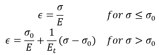
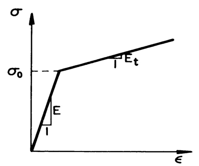
Figure 2: Elastic-linear work-hardening stress-strain curve [1]
1.1.3. Elastic-exponential hardening model
Consider a power expression of the type:
where k and n are two characteristic constants of the material to be determined to best fit the experimentally obtained curve. If ![]() represents the total strain, the curve should pass through the point representing the yield stress and the corresponding elastic strain. The power expression should be used only in the strain-hardening range.
represents the total strain, the curve should pass through the point representing the yield stress and the corresponding elastic strain. The power expression should be used only in the strain-hardening range.
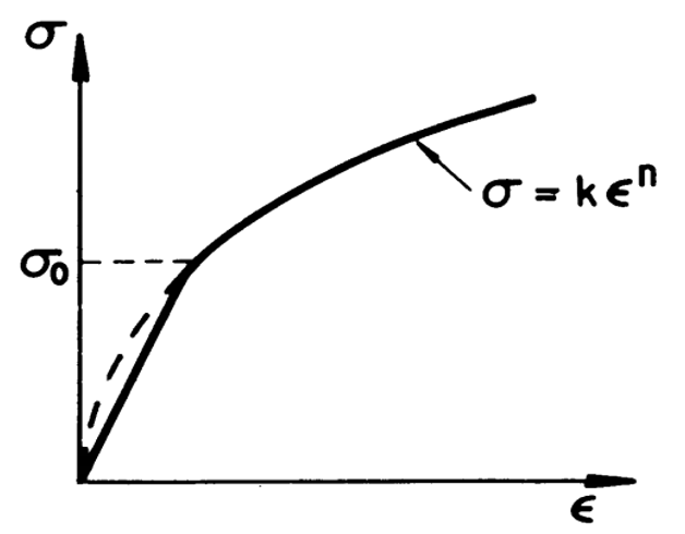
Figure 3: Elastic-exponential hardening stress-strain curve [1]
1.1.4. Ramberg-Osgood model
The nonlinear stress-strain curve as shown in figure 4 has the following expression:
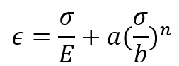
in which a, b, and n are material constants. The initial slope of the curve takes the value of Young’s modulus E at ![]() , and decreases monotonically with increasing loading. Since the model has three parameters, it allows for a better fit of real stress-strain curves.
, and decreases monotonically with increasing loading. Since the model has three parameters, it allows for a better fit of real stress-strain curves.
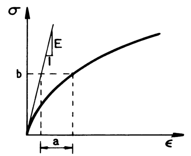
Figure 4: Ramberg-Osgood stress-strain curve [1]
2. Abaqus Plasticity model (Modeling)
Abaqus provides a comprehensive library of plasticity models that cover a wide range of material behaviors. These models are shown in Figure 5.
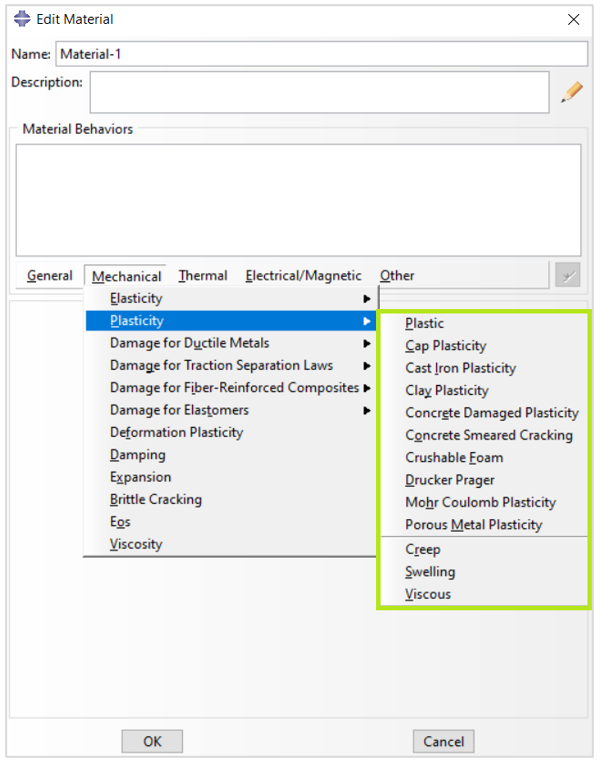
Figure 5: Abaqus plasticity models for different material behaviors
As you can see there are several options for modeling plasticity in Abaqus which are out of the scope of this discussion. In this post, we will introduce the first option which is ‘Plastic’, and uses Mises or Hill yield surfaces with associated plastic flow. It is one of the most common models you may use in your simulations.
2.1. Plastic Region Definition in Abaqus
In Abaqus/CAE to define this plasticity model you must do as following:
- Go to the “Property” module
- Define a Material
- Mechanical> Plasticity> Plastic
After that, you must provide some data that we will discuss about them here. These data are shown in figure 6.
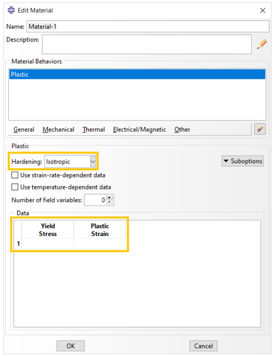
Figure 6: Data for plastic definition in Abaqus
You need to determine the hardening and enter the plastic region data including plastic strain and its corresponding yield stress in this window.
Let’s first determine how to enter the appropriate data for the plastic region.
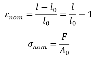
When defining plasticity data in Abaqus, you must use true stress and true strain. Abaqus requires these values to interpret the data in the input file correctly. However, quite often material test data are supplied using values of nominal stress and strain. In such situations, you must convert the plastic material data from nominal stress and strain to true stress and strain.
The relationship between true strain and nominal strain is as follows:
![]()
The relationship between true stress and nominal stress is formed by considering the incompressible nature of the plastic deformation and assuming the elastic volumetric deformation is negligible. So, the relationship between true stress and nominal stress and strain is:
![]()
Where in the previous relations, ![]() and
and ![]() can be expressed as:
can be expressed as:
The strains provided in material test data used to define the plastic behavior are not likely to be the plastic strains in the material. Instead, they will probably be the total strains in the material. You must decompose these total strain values into the elastic and plastic strain components. The plastic strain is obtained by subtracting the elastic strain, defined as the value of true stress divided by Young’s modulus, from the value of total strain (Figure 7). This relationship is written as:
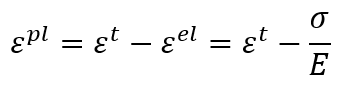
Where ![]() is true plastic strain,
is true plastic strain, ![]() is true total strain,
is true total strain, ![]() is true elastic strain,
is true elastic strain, ![]() is true stress, and E is Young’s modulus.
is true stress, and E is Young’s modulus.
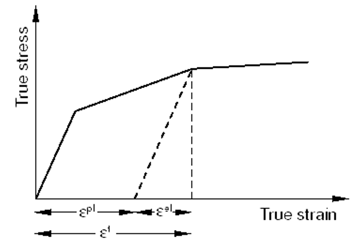
Figure 7: Strain components in a deformation
Abaqus connects your stress-strain data pairs with a series of straight-line segments to form a continuous, piecewise linear plasticity curve. You can use any number of data pairs to approximate the actual material behavior; therefore, it is possible to get a very close approximation of the actual material behavior.
Let’s implement the previous concepts in an example.
2.1.1. Example of converting material test data to Abaqus input
The stress-strain curve in figure 8 will be used as an example of how to convert the test data defining a material’s plastic behavior into the appropriate input format for Abaqus.
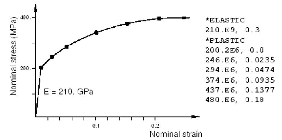
Figure 8: Elastic-plastic material behavior and corresponding Abaqus input data
The first step is to use the equations relating the true stress to the nominal stress and strain and the true strain to the nominal strain to convert the nominal stress and nominal strain to true stress and true strain. Once these values are known, the equation relating the plastic strain to the total and elastic strains which were shown earlier can be used to determine the plastic strains associated with each yield stress value. The converted data are shown in table 1.
Table 1: Converting nominal stress and strain to true stress and strain
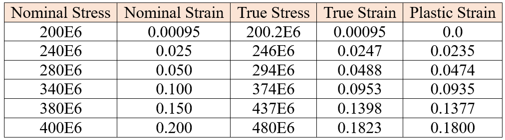
As you can see in figure 8, the ‘True Stress’ and ‘Plastic Strain’ columns of this table are entered as Abaqus input data for the plastic definition.
It’s good for you to obtain the values in table 1 from the nominal stress and strain as a practice using the mentioned relations.
Now let’s see what are the different hardening types you can define in Abaqus plastic.
In Abaqus, a perfectly plastic material (with no hardening) can be defined, or work hardening can be specified. Isotropic hardening is available in both Abaqus/Standard and Abaqus/Explicit; Johnson-Cook hardening is available only in Abaqus/Explicit. In addition, Abaqus provides kinematic hardening for materials subjected to cyclic loading.
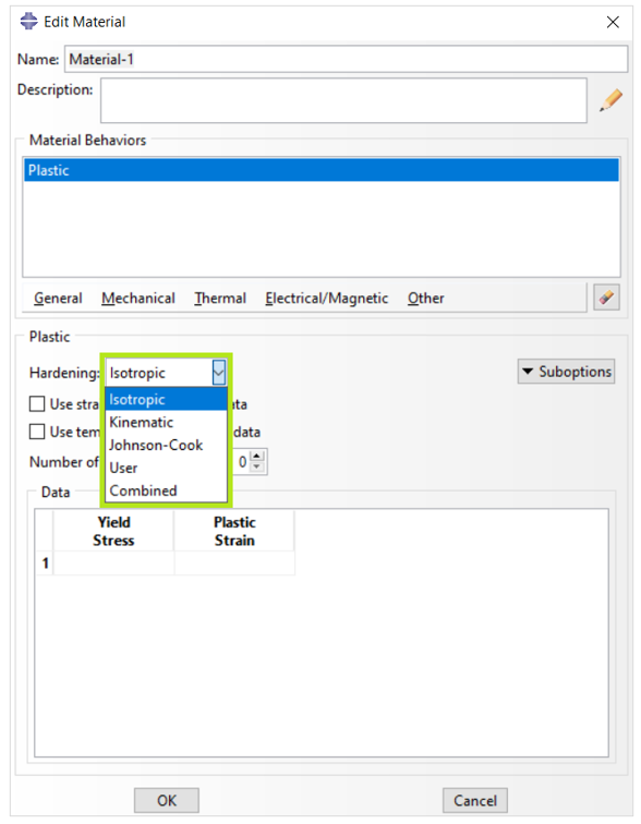
Figure 9: Different hardening types for Abaqus plasticity
2.1.2. Perfect Plasticity | Elastic perfectly plastic Abaqus
Perfect plasticity means that the yield stress does not change with plastic strain. It can be defined in tabular form for a range of temperatures and/or field variables; a single yield stress value per temperature and/or field variable specifies the onset of yield.
Imagine the only inelastic material data available for steel are its yield stress (380 MPa) and its strain at failure (0.15). You decide to assume that the steel is perfectly plastic: the material does not harden, and the stress can never exceed 380 MPa as in figure 10.
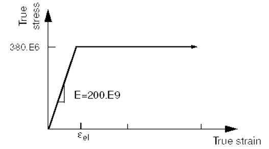
Figure 10: Stress-strain behavior for the perfectly plastic steel
The initial yield stress at zero plastic strain is 380 MPa. Since you are modeling the steel as perfectly plastic, no other yield stresses are required (Figure 11).
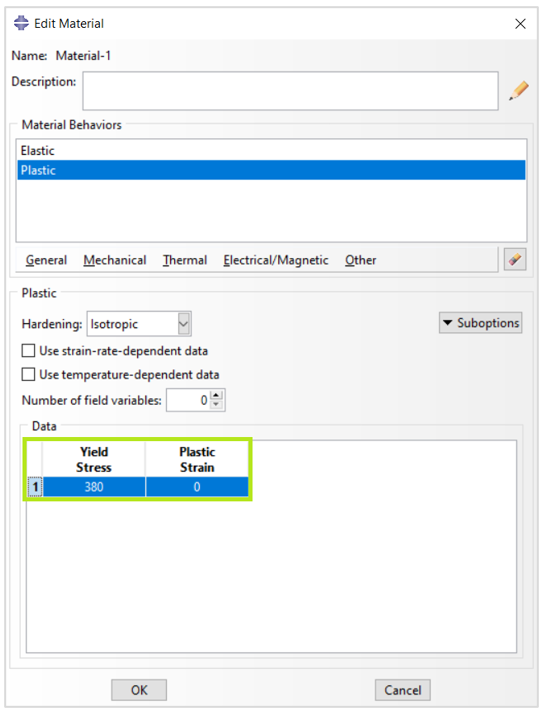
Figure 11: Define an elastic-perfectly plastic material
2.1.3. Isotropic Hardening
For a perfectly plastic material, the equation for the fixed yield surface has the form, ![]() , where k is a constant. The simplest work-hardening rule is based on the assumption that the initial yield surface expands uniformly without distortion and translation as plastic flow occurs, as shown schematically in figure 12. The size of the yield surface is now governed by the value
, where k is a constant. The simplest work-hardening rule is based on the assumption that the initial yield surface expands uniformly without distortion and translation as plastic flow occurs, as shown schematically in figure 12. The size of the yield surface is now governed by the value ![]() , which depends upon plastic strain history.
, which depends upon plastic strain history.
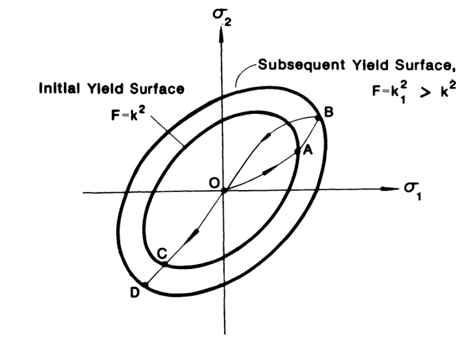
Figure 12: Subsequent yield surface for isotropic-hardening material [1]
The isotropic hardening model is simple to use, but it applies mainly to monotonic loading without stress reversals. So, it cannot account for the Bauschinger effect exhibited by most structural materials.
If isotropic hardening is defined, the yield stress, ![]() , can be given as a tabular function of plastic strain and, if required, of temperature and/or other predefined field variables. The yield stress at a given state is simply interpolated from this table of data, and it remains constant for plastic strains exceeding the last value given as tabular data.
, can be given as a tabular function of plastic strain and, if required, of temperature and/or other predefined field variables. The yield stress at a given state is simply interpolated from this table of data, and it remains constant for plastic strains exceeding the last value given as tabular data.
2.1.4. Kinematic Hardening
The kinematic hardening rule assumes that during plastic deformation, the loading surface translates as a rigid body in stress space, maintaining the size, shape, and orientation of the initial yield surface (Figure 13).
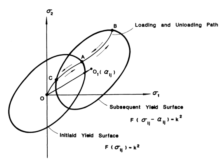
Figure 13: Subsequent yield surface for kinematic-hardening material [1]
As a consequence of assuming a rigid-body translation of the loading surface, the kinematic hardening rule predicts an ideal Bauschinger effect for a complete reversal of loading conditions.
Two kinematic hardening models are provided in Abaqus to model the cyclic loading of metals. The linear kinematic model approximates the hardening behavior with a constant rate of hardening. The more general nonlinear isotropic/kinematic model will give better predictions but requires more detailed calibration.
To specify the nonlinear combined isotropic/kinematic model, you must select the ‘Combined’ hardening.
2.1.5. Johnson-Cook Isotropic Hardening
Johnson-Cook hardening is a particular type of isotropic hardening in Abaqus/Explicit where the yield stress is given as an analytical function of equivalent plastic strain, strain rate, and temperature. This hardening law is suited for modeling the high-rate deformation of many materials including most metals.
For detailed information about Johnson-Cook hardening, we recommend to see the following link:
Introduction to Abaqus Johnson-Cook Model: Accurately Model High-Strain rate Events
2.1.6. User Hardening
In Abaqus/Standard the yield stress for isotropic hardening, ![]() , can alternatively be described through the user subroutine UHARD.
, can alternatively be described through the user subroutine UHARD.
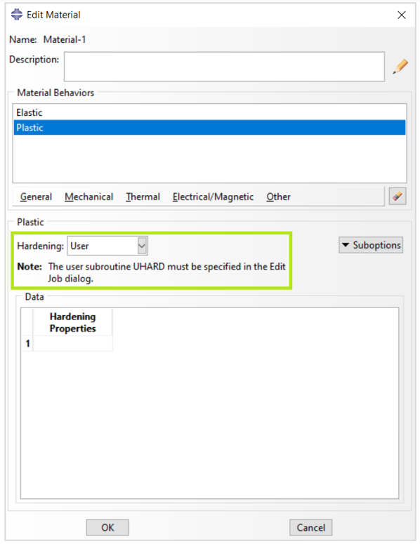
Figure 14: Defining User hardening in Abaqus plasticity
For detailed information about UHARD subroutine, we recommend to see the following link:
UHARD Subroutine (VUHARD Subroutine) in ABAQUS
What an amazing way we came through! Time to summarize what we have learned in this way.
3. Summary
We started our discussion by clarifying the importance of plasticity subject. Then we introduced some of the common plastic behaviors in materials. In advance, we talked about Abaqus plasticity and some of the capabilities of Abaqus to model plasticity.
In Abaqus, plasticity is implemented using a variety of material models, each of which is tailored to capture the specific behavior of a particular material or class of materials.
An important aspect of Abaqus plasticity is the use of hardening laws to describe the evolution of the material’s yield stress with plastic strain. Abaqus provides several built-in hardening laws, including isotropic, kinematic, and mixed hardening, as well as the ability to define user-defined hardening laws.
In the end, we appreciate for reading this article. Don’t forget to leave us your comments about this article to improve our content quality. Wish you the Best.
4. Users ask these questions
Defining the plastic properties is a common thing in Abaqus and so there are a lot of questions regarding this matter in many platforms and social media; therefore, we decided to answer a few of them.
I. Plastic region
Q: Having a perfect plastic region doesn’t make any convergence issues?
A: To avoid convergence problems, add a slight slope in the perfect plastic region. You can add a perfect plastic region like in figure 1. But you may encounter a convergence issue because the plastic strain is increasing in this model while the stress remains at the same value. Therefore, add a slight slope to avoid this issue (see figure 2). Note that all values in figures are just for example and don’t have to be true.
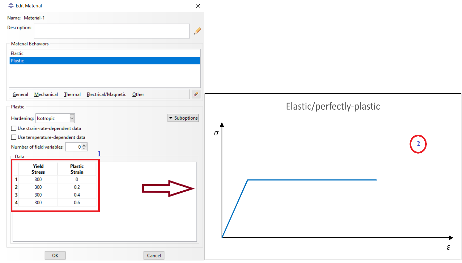
Figure 1: Perfect plastic region
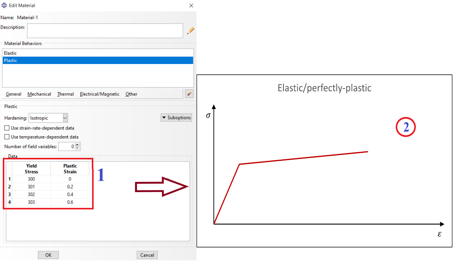
Figure 2: Perfect plastic region with slight slope