
Abaqus Standard vs Explicit Explained: Pick the Right One
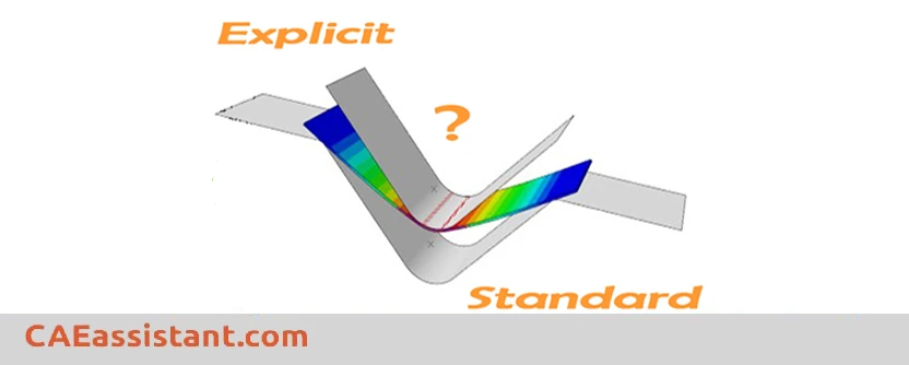
Which one should you use: Abaqus Standard or Abaqus Explicit? If you’ve run into this question while working in Abaqus, you’re definitely not alone.
Abaqus gives you two powerful solvers for finite element analysis—Standard (Implicit) and Explicit. But when you’re dealing with complex simulations, knowing which one to use isn’t always obvious.
Think of it this way:
The Abaqus Standard solver works like a cautious planner. It checks that everything balances—loads, reactions, deformations—before moving to the next step. This makes it perfect for static problems or slower nonlinear simulations.
In contrast, the Abaqus Explicit solver is built for speed. It skips the heavy balancing act at every step and pushes the simulation forward quickly. That’s why it shines in dynamic events like impacts, crashes, or sudden contact.
This blog breaks down the core in the Abaqus Standard vs Explicit debate. You’ll learn:
-
How each solver approaches the problem
-
The types of scenarios each one is best suited for
-
Which solver saves you time (and when)
By the end, you’ll have a clear understanding of which Abaqus solver to choose—and why it matters.
6 hours of professional, in-depth, yet beginner-friendly tutorials, with hands-on workshops to help you apply what you learn. The Abaqus for beginners package is all you need to start mastering Abaqus and become a skilled FEA analyst.
 |
|
1. What Are Implicit and Explicit Methods?
Before we compare Abaqus Standard vs Explicit, it’s useful to understand what implicit and explicit actually mean in simulation terms.
These terms refer to how the solver handles time and motion—specifically, how it steps forward through a simulation.
Implicit Method (Used in Abaqus Standard)
In an implicit method, the solver checks balance at every time step. It solves a system of equations to make sure forces and displacements are in equilibrium. This often involves iterative methods like Newton-Raphson, especially in nonlinear problems.
It’s more stable and allows larger time steps—but takes more computational effort per step.
Want to learn how Newton-Raphson works in detail? Check out this simple breakdown.
Explicit Method (Used in Abaqus Explicit)
An explicit method doesn’t solve equations for balance at every step. Instead, it calculates accelerations directly from the applied forces and updates the motion step by step.
It’s fast and efficient for very short time steps—especially useful in high-speed or complex contact problems.
2. What is Abaqus Standard (Implicit) Solver?
Abaqus Standard, also known as the implicit solver, is designed for simulations where the system needs to find equilibrium at each step.
This solver uses an implicit time integration method, meaning it solves a set of equations that balance forces, displacements, and constraints. It typically uses Newton-Raphson iteration to converge on the solution—especially for nonlinear problems.
In Abaqus, an equilibrium solution is the state where internal forces (stresses) balance external forces (applied loads), indicating stability without further movement. For equilibrium:
- Force equilibrium: Total external forces must equal internal forces.
- Moment equilibrium: The sum of all moments around any point or axis must be zero.
Abaqus checks for equilibrium by solving for displacements and stresses, which is crucial in static analyses focusing on the final deformed shape and stress distribution.
When Should You Use Abaqus Standard?
Use Abaqus Standard when your simulation involves:
-
Static problems (e.g. structural loading, thermal steady-state)
-
Quasi-static nonlinear problems (e.g. contact or plasticity under slow loading)
-
Abaqus dynamic implicit simulations (e.g. vibration, fatigue, or stability)
-
Coupled field problems (e.g. thermal-mechanical analysis)
It’s especially powerful for accurate long-term behavior in structures, where equilibrium matters more than speed.
Strengths of Abaqus Standard
-
Unconditionally stable: You can use larger time increments without worrying about numerical instability.
-
Ideal for equilibrium-based problems: Great for slow or static loads where final balance is key.
-
Excellent for nonlinear behavior: Handles large deformations, plasticity, contact, and creep with precision.
-
Supports advanced analysis types: Like buckling, frequency extraction, and thermal-mechanical coupling.
Limitations of Abaqus Standard
-
Computationally intensive: Solving equilibrium iteratively takes time, especially for nonlinear problems.
-
Can struggle with severe contact: Too many contact interactions can slow convergence.
-
Less efficient in high-speed dynamics: For crash-like simulations, this solver is often too slow or unstable.
If your problem is more about accuracy and balance over time, and not sudden impacts, Abaqus Standard (or Abaqus Implicit) is the better choice.
Think of it as a solver that prioritizes control and stability, even if it means taking a little longer to get there.
Abaqus Standard comes with a range of implicit analysis procedures, each crafted for different kinds of problems. Here’s an overview of the key Abaqus implicit steps, organized by the type of analysis and procedure:
2.1. Static, General Step
The Static General procedure in Abaqus Standard is widely used for static analysis of structures, ideal for gradual loads or boundary conditions until equilibrium is reached. It helps analyze structural deformation, stress distribution, and static loads in both linear and nonlinear systems.
When setting up a static general procedure, the Edit Step dialog box displays three tabs—Basic, Incrementation, and Other (fig 1)—allowing you to customize settings like the time period, maximum increments, increment size, load variation, and geometric nonlinearity. We explore these options to tailor the procedure!
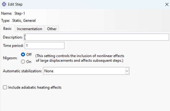
Figure 1: Static, general procedure
You can easily set up important settings like “Nlgeom” and “stabilization” using the Basic tabbed page. Let’s walk through it step by step!
- Choose your Nlgeom option:
– If you select “Off,” you’ll be running a geometrically linear analysis for this step.
– If you’d like ABAQUS Standard to factor in geometric nonlinearity, select “On.” Just remember, once you turn Nlgeom on, it stays active for all the next steps!
- If you’re expecting any local instabilities (local instabilities refer to situations where a structure or a component experiences sudden, uncontrolled deformations in a localized region.) like surface wrinkling or local buckling, go ahead and toggle on Use “Stabilization” (fig.2). This feature helps ABAQUS/Standard stabilize those tricky areas by applying damping throughout the model.
- If you have turned on Use Stabilization, click the arrow of the combo box to choose a method for defining the damping factor (fig 2):
– You can opt for the dissipated energy fraction, which allows ABAQUS/Standard to calculate the damping factor based on a fraction you provide. Just enter the value in the adjacent field.
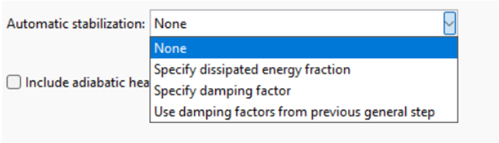
Figure 2: Apply stabilization
- If you’re conducting an adiabatic stress analysis (Adiabatic stress analysis studies stress and temperature changes in a material or structure under conditions without heat exchange between the system and its surroundings.), don’t forget to toggle on Include Adiabatic Heating Effects (fig 3). This is only relevant for isotropic metal plasticity materials that have a Mises yield surface.
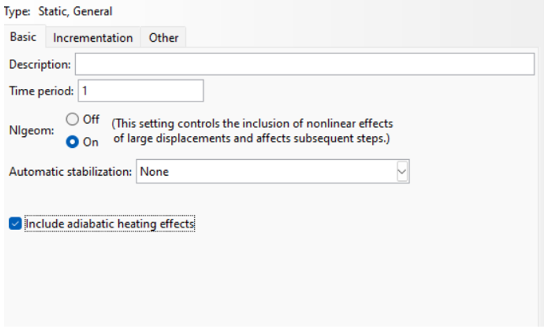
Figure 3: apply adiabatic heating
Next in the Incrementation tab to easily configure your increment size and the maximum number of increments. Here’s a guide to help you through the process:
- Automatic Type:
– If you prefer some flexibility, select Automatic. This lets ABAQUS Standard decide on the best increment sizes for efficiency (fig 4).
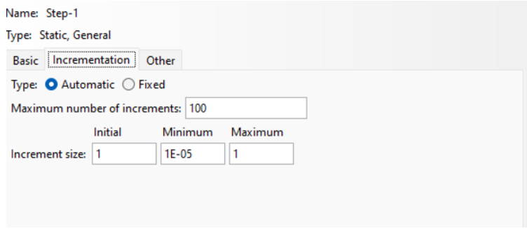
Figure 4: Choose Automatic type
– In the “Maximum number of increments” field, you can set an upper limit for how many increments are allowed in this step. Just keep in mind that if this limit is exceeded, the analysis will stop before ABAQUS Standard finds the complete solution.
– Initial: Enter your starting time increment here.
– Minimum: Enter the smallest time increment you’d like to allow.
– Maximum: Set your upper limit for the time increment here.
2 – Fixed Type:
– Want full control? Go for Fixed! This option lets you set a constant increment size that will be used throughout the step (fig 5).
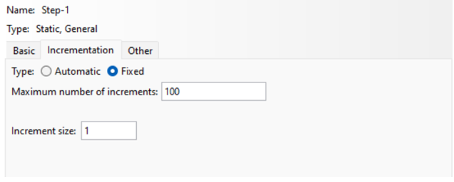
Figure 5: Apply Fixed incrementation type
When we say “constant time increment size,” we mean that the time it takes to increase a number by a fixed amount (usually by 1) doesn’t change, no matter the number’s value. Constant time size ensures that your runs efficiently, even as the number of size of the data increases. For that’s matter Simply enter the constant time increment you want in the Increment size field, and you’re all set!
Here are the essentials for making the right choice in full.
- Open the Edit Step dialog box and navigate to the Other tab.
- Choose Your Equation Solver Method:
The Equation Solver Method in the general solver refers to the approach used to solve the system of equations generated during the finite element analysis (FEA) process. These equations represent the balance of forces or energy in the system based on the problem’s governing equations (e.g., equilibrium, compatibility, and constitutive equations). The Equation Solver Method includes the following (figure 6):
– Direct: This is a direct solution method that solves the system of equations by explicitly factoring the system’s stiffness matrix. It computes the solution vector directly through a matrix factorization process (The matrix factorization process involves decomposing linear algebraic equations from finite element analysis into simpler forms for efficient solving. It’s a crucial part of direct solvers (Full Matrix Solver) and significantly affects the speed and efficiency of solving these equations.).
– Iterative: The iterative solver approaches the system of equations by progressively refining an initial guess of the solution through a series of iterations. The solution is computed by minimizing the residual error in each iteration.
– Use Solver default: Let ABAQUS/Standard decide whether to use a symmetric or unsymmetric matrix.
– Unsymmetric: The unsymmetric storage and solution scheme in ABAQUS/Standard is used when the stiffness matrix is unsymmetric, commonly in nonlinear problems, dynamic analyses, or specific boundary conditions. This approach allows for more flexible handling of the matrix, utilizing iterative solvers and memory-intensive methods to solve equations despite the lack of symmetry.
– Symmetric: Keep it to symmetric storage and solutions only.
You can learn more about Abaqus Implicit and Abaqus Explicit and the difference between them, you can find valuable info in the lesson 4 of the Abaqus for beginners package.

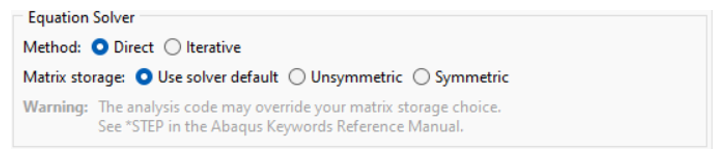
Figure 6: Equation Solver Method
- Handle Severe Discontinuities:
Click the arrow next to the “Convert severe discontinuity iterations” field and choose how to approach severe discontinuities during your analysis (fig 7):
– Off: Start a new iteration if any severe discontinuities pop up.
– On: Let ABAQUS estimate residual forces related to these discontinuities, checking if equilibrium tolerances are being met. This might allow for convergence in some cases.
– Propagate from the previous step: Use a value from the last general analysis step.
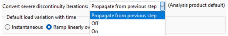
Figure 7: Handle Severe Discontinuities
- Extrapolate Previous State:
Click the arrow next to the “Extrapolation of the previous state at the start of each increment” field and select a method. The method determines how Abaqus predicts the starting point (initial guess) for the solution in the current increment based on the results from the previous increment. A good initial guess can significantly speed up convergence in nonlinear problems (fig 8).
– Linear: Abaqus extrapolates the displacement and stress states linearly from the previous increment to predict the initial conditions for the current increment. This is typically more efficient and helps accelerate convergence, especially when the system is behaving smoothly.
– Parabolic: Use a quadratic extrapolation based on the last two increments.
– None: Skip the extrapolation altogether.
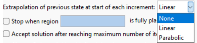
Figure 8: Extrapolate Previous State
2.2. Abaqus Dynamic Implicit
“Abaqus Dynamic Implicit” describes a time integration method in ABAQUS Standard for dynamic problems. It computes next time step values using current and previous values, allowing for larger time steps than explicit integration. However, it requires solving nonlinear equations at each step, making it suitable for structural problems where stability and time step control are crucial.
When you’re setting up a “dynamic, implicit” procedure in ABAQUS, you’ll see three tabs in the step editor: Basic, Incrementation, and Other. These tabs let you adjust important settings like the time period, increment size, and solver preferences for your analysis.
Basic Tab Settings (fig 9):
The Basic tab settings are all like the ones in the “Static, General” step. But let’s see its applications.
1. Application:
- Transient fidelity specifically relates to how accurately the dynamic implicit Abaqus solver can capture a system’s time-dependent behavior, especially under dynamic loading conditions, such as impacts, vibrations, or other transient effects. It reflects how well the solver can model the time evolution of quantities such as displacement, velocity, acceleration, and stresses during a dynamic event.
- Moderate dissipation involves adding a controlled amount of artificial damping to the system. This helps to remove high-frequency oscillations or numerical noise that can arise in dynamic problems, particularly those with rapid loading or unstable modes of vibration.
- Quasi-static in Implicit Dynamic in Abaqus refers to using a dynamic solver to handle time-dependent nonlinear behavior but neglecting inertial effects. Thus, the problem is effectively treated as a slow-static problem while still benefiting from the robustness of implicit integration and the ability to model complex nonlinearities.
2. For adiabatic stress analysis (only for isotropic metal plasticity with a Mises yield surface), toggle Include adiabatic heating effects.
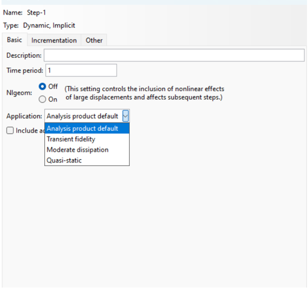
Figure 9: Dynamic Implicit basic tab settings
Incrementation Tab Settings are also like the ones in the “Static, General” step. In this step, optionally, you can toggle on Suppress half-step residual calculation to speed up the solution.
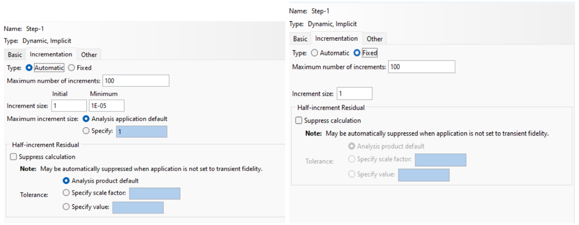
Figure 10: Incrementation Tab Settings
Other Tab Settings (fig 11):
- Go to the Other tab in the Edit Step dialog box.
- Matrix Storage:
- Using solver default allows ABAQUS to choose the best storage scheme.
- Symmetric or Unsymmetric restricts ABAQUS to these storage schemes.
- Solution Technique:
- Choose Full Newton or Quasi-Newton for solving nonlinear equations. Quasi-Newton is faster for large systems with little stiffness change.
- If using Quasi-Newton, set the number of iterations allowed before reforming the matrix (default is 8, max is 25).
- Handling Severe Discontinuities:
- Off forces a new iteration if discontinuities occur.
- On estimates forces related to severe discontinuities and may adjust the solution method.
- Propagate from the previous step uses the value from the prior step.
- Load Variation with Time:
- Instantaneous applies the full load at the start and keeps it constant.
- Ramp Linearly increases the load from the previous step to full magnitude.
- Extrapolation of Previous State:
- Linear uses a simple linear guess for the current increment.
- Parabolic uses a more advanced quadratic guess.
- For Dynamic Steps, ABAQUS calculates accelerations by default at the start. If you prefer a simpler approach:
- Bypass initial acceleration calculations will set accelerations to zero in the first dynamic step, or continue from the previous step if it was dynamic.
- Accept Solution After Maximum Iterations: If you use Fixed time incrementation, you can accept a solution even if it hasn’t reached equilibrium. This option is only recommended when you fully understand the results.
Once you’ve adjusted all the settings, simply click OK to save your changes and close the dialog.
Learn more about Newton-Raphson Technique in this article: “Abaqus nonlinear analysis VS linear analysis“
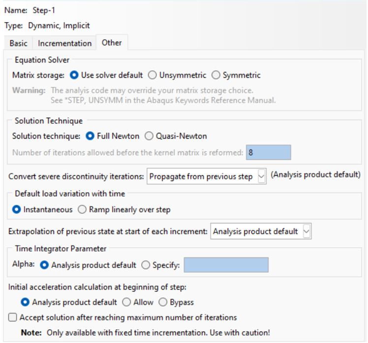
Figure 11: Other Tab Settings
By following these steps, you can ensure your dynamic analysis is set up to meet your specific needs, whether you’re focusing on accuracy, computational efficiency, or both.
3. What is the Abaqus Explicit Solver?
Abaqus Explicit is built for fast, high-energy events—the kinds where things crash, explode, or deform in milliseconds.
It uses an explicit time integration method, which means it doesn’t solve complex equations at every time step. Instead, it calculates the motion directly based on known values of forces and accelerations.
This makes it incredibly fast for very short time steps—perfect for events that happen quickly and involve lots of contact or failure.
When Should You Use Abaqus Explicit?
Use Abaqus Explicit when your simulation involves:
-
High-speed dynamics (e.g. impact, crash, drop tests)
-
Abaqus dynamic explicit scenarios (e.g. blast, penetration, metal forming)
-
Severe contact and large deformation (e.g. airbags, crushing, cutting)
-
Material failure or erosion (e.g. fracture, element deletion)
-
Short-duration events (e.g. milliseconds)
It’s also useful when the Abaqus implicit method fails to converge—like in cases with complicated contact interactions.
Strengths of Abaqus Explicit
-
No need to solve equations per step: Each time step is direct and fast.
-
Excellent for complex contact: Easily handles parts that slide, collide, or separate suddenly.
-
Great for failure and large deformation: Simulates materials breaking, tearing, or flowing.
-
Supports mass scaling: You can speed up simulations without losing accuracy—if done right.
-
Stable for short time steps: Perfect for fast events.
Limitations of Abaqus Explicit
-
Conditionally stable: Requires very small time steps to remain accurate and stable.
-
Not efficient for slow simulations: Overkill for long, slow processes like creep or static loading.
-
Time-consuming for long durations: Even if each step is fast, thousands of tiny steps can take a while.
If your simulation is all about speed, impact, and complexity, go with Abaqus Explicit. It’s built for chaos—fast-moving events with contact, breakage, or violent motion.
Think of it as a solver that trades calculation effort for speed, moving fast step by step without solving the whole system each time.
Here are the main settings for explicit solvers in Abaqus:
3.1. Abaqus Dynamic Explicit
An Abaqus dynamic Explicit step is a type of analysis step used to simulate highly dynamic, transient problems involving large deformations, high strain rates, or complex contact interactions. Unlike implicit methods, explicit methods directly solve the equations of motion and are well-suited for problems involving impacts, crashes, explosions, or other fast-changing events.
Let’s explore the configuration options available in the Edit Step dialog box for setting up a Dynamic, Explicit procedure in Abaqus! Here’s a guide to help you navigate the different tabs and make the most of your settings:
Basic Tab: Like the general statics, this Tab is designed to solve problems (Fig 12).
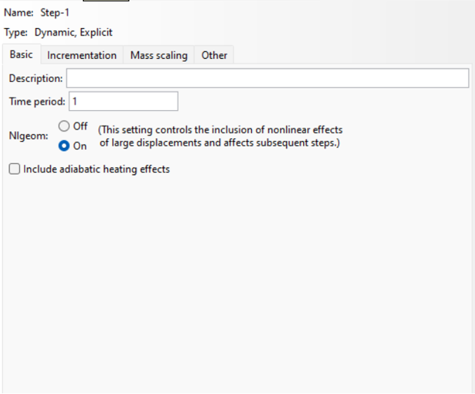
Figure 12: Basic settings for dynamic Explicit Abaqus
Incrementation Tab:
Like other solvers, the incrementation tab is divided into two types: fix and automatic.
Automatic incrementation is essential when simulating problems with complex contact interactions (e.g., impacts or collisions), where large changes in forces and velocities occur rapidly (fig 13).
- A stable increment estimator is used to automatically determine the maximum stable time increment for each analysis step. This time increment is critical because it controls the rate at which the solution progresses through time. The increment must be small enough to satisfy stability criteria, particularly for problems involving high-speed events, large deformations, or complex interactions.
- Abaqus provides several methods to improve the selection of time increments during explicit dynamic analysis. The goal is to achieve a balance between computational efficiency and accuracy while maintaining the stability of the solution. To use this feature you must enable the “improved Dt method”.
- You can define a maximum time increment for the analysis. This is useful to control how finely the time steps are taken. Smaller time increments may improve accuracy but increase computational cost.
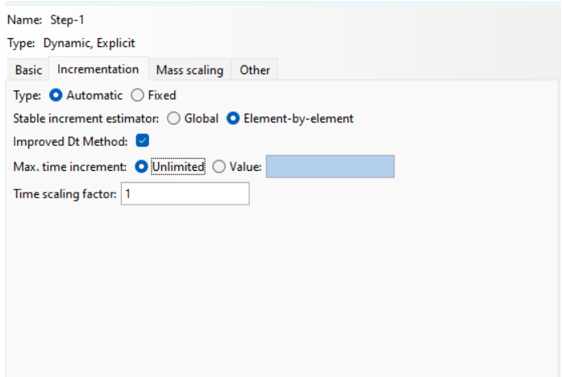
Figure 13: Automatic incrementation in Abaqus Explicit
The fixed type in the explicit solver is like the fixed type in general implicit so that you could see in the static, General section.
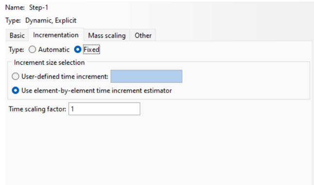
Figure 14: fixed type in dynamic, Explicit
Mass Scaling Tab:
Mass scaling is often used to artificially speed up the simulation by scaling the mass matrix. This is particularly useful when you are simulating a very long or complex dynamic process but want to make the simulation more computationally efficient (fig 15).
- Mass Scaling:
-
- Mass scaling can be used to increase the mass of certain elements in the model, which effectively reduces the time steps needed for stable results.
- You can specify the scaling factor, the regions of the model to apply mass scaling, and the magnitude of the scaling.
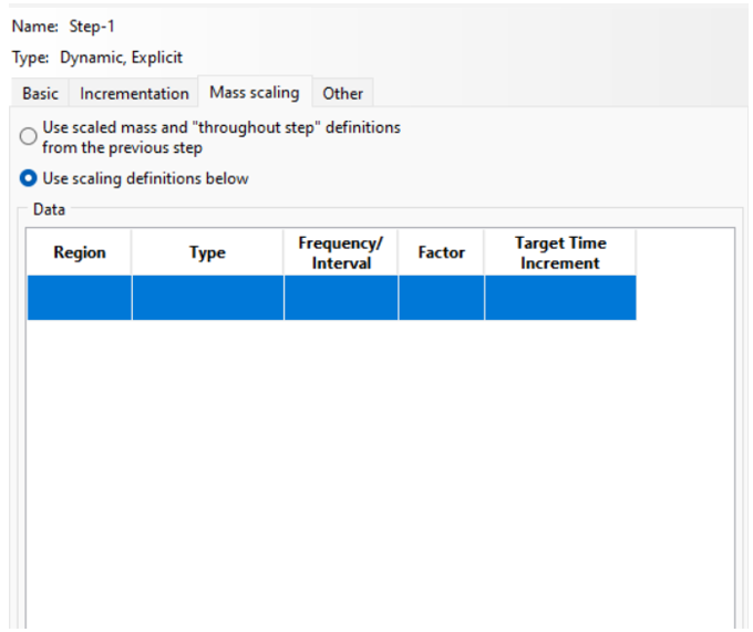
Figure 15: mass scaleing
Note: While mass scaling can make simulations more computationally efficient, it should be used with care, as it can alter the physical behavior of the system, especially if applied in a non-physical manner (e.g., scaling mass in regions that experience little motion).
Other Tab:
This tab has an advanced option that can affect the behavior and performance of the simulation.
- Bulk Viscosity(fig 16):
-
- Bulk viscosity helps control high-frequency oscillations in the results that may arise in explicit dynamics simulations. It applies a damping force proportional to the rate of change of the velocity field.
- You can configure the bulk viscosity parameter to smooth out high-frequency noise in the solution, particularly in simulations with shock waves or high deformation rates.
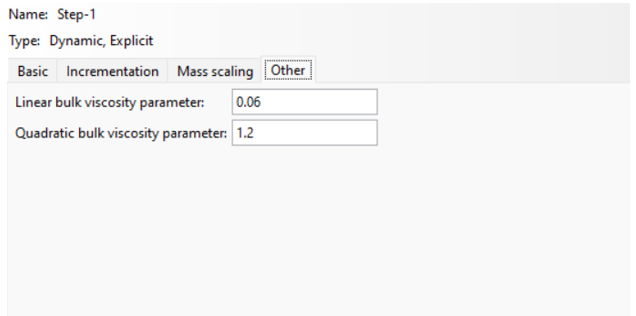
Figure 16: other tab for Dynamic, Explicit
4. Abaqus Standard vs Explicit: A Side-by-Side Comparison
First, I have to say that there are no differences between Standard and Implicit. In fact, these are two names for one solver. The main discussion is about Abaqus Implicit and Explicit solvers.
These solvers are based on two approaches in FEM analysis, namely implicit (for Abaqus/Standard) and explicit. The distinction between the two different numerical approaches makes it possible to understand which solver to use.
Now that you understand what Abaqus Standard (Implicit) and Abaqus Explicit solvers do individually, let’s put them head to head.
When choosing between them, it all comes down to your simulation’s needs: speed, accuracy, contact complexity, stability, or long duration.
In the case of the implicit method, equilibrium is enforced between externally applied load and internally generated reaction forces at every solution step (Newton Raphson method).
In the case of the explicit method, there is no enforcement of equilibrium. But this does not mean that explicit is not accurate. You can minimize its deviation from equilibrium to almost zero by increasing the number of solution steps, i.e. reducing the time step size.
We can list the main differences below:
Implicit is unconditionally stable.
Implicit schema is incremental as well as iterative. However, explicit schema is only incremental (Abaqus Increment).
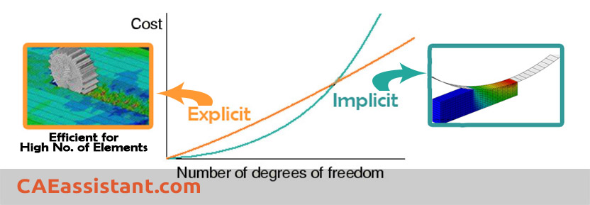
In terms of cost per Increment, it is costly for implicit and cheaper for explicit. Disk space and memory usage are typically much smaller than that for implicit. The explicit method shows great cost savings over the implicit method as the model size increases:
Therefore, Abaqus Standard (or implicit) must iterate to determine the solution to a nonlinear problem but Abaqus/Explicit determines the solution without iterating by explicitly advancing the kinematic state from the previous increment.
Here’s a simple breakdown of how they compare in key areas:
| Feature | Abaqus Standard (Implicit) | Abaqus Explicit |
|---|---|---|
| Time Integration | Implicit method | Explicit method |
| Solver Type | Solves equilibrium equations (e.g., Newton-Raphson) | Direct calculation without solving equations |
| Typical Use Cases | Static, quasi-static, slow dynamics, thermal-mechanical coupling | High-speed impacts, crash tests, forming, explosions |
| Convergence Requirement | Yes – requires iterative convergence | No – direct solution, no iteration needed |
| Stability | Unconditionally stable | Conditionally stable – small time steps required |
| Time Step Control | Automatically adjusted | Must be manually controlled or mass-scaled |
| Computational Cost | Fewer steps, but each step is expensive | Many steps, but each step is fast |
| Best For | Long-duration accuracy, complex material behavior | Short-duration, high-deformation, complex contact |
| Ease of Setup | More parameters to tune, convergence-sensitive | Easier to set up for contact-rich problems |
Now, let’s get into some details to better understand the Abaqus Standard VS Explicit:
- Dynamic Effects each solver has;
- how each solver handle contact;
- and special features for each solver.
4.1. Dynamic Effects: Motion, Forces, and Stability
How your simulation handles motion and inertia can completely change the results. Here’s how Abaqus Standard and Abaqus Explicit approach dynamic effects:
Abaqus Standard (Implicit)
By default, Abaqus Standard solves for static equilibrium—where all forces balance out, and nothing accelerates. You can also run Abaqus dynamic implicit simulations to include inertia and damping. But if you’re running a purely static analysis:
-
Every part must be fully constrained (connected to the ground in all directions).
-
Rigid body motion isn’t allowed—it will cause the solution to fail.
-
You can’t rely on inertia to help reach equilibrium.
-
If your system needs to “settle” (e.g., through vibrations or internal energy release), you’ll need to artificially help it—like applying damping.
In short: if your system doesn’t naturally reach static equilibrium, the implicit solver won’t solve it unless you guide it.
Abaqus Explicit
Abaqus Explicit always solves for dynamic equilibrium, based on Newton’s second law:
Force = Mass × Acceleration.
That means:
-
Vibrations and oscillations are expected, even in what feels like a static problem.
-
Time is real—how fast you apply loads matters.
-
You can’t just ignore dynamic effects; they’re always there.
-
If you don’t want dynamic effects to influence results (e.g., you’re simulating a slow press), you need to apply the load very slowly.
Mass scaling is often used here. You can artificially increase the mass of the system to take larger time steps and speed up the simulation. But be careful—too much scaling can introduce nonphysical results by adding unwanted inertia.
| Category | Abaqus Standard (Implicit) | Abaqus Explicit |
|---|---|---|
| Type of Equilibrium | Static or Dynamic | Always Dynamic |
| Handles Rigid Body Motion | ❌ Not allowed unless constrained | ✅ Naturally handled |
| Internal Energy to Kinetic Energy | ❌ Needs damping | ✅ Happens naturally |
| Load Rate Importance | Less critical | Critical (affects results) |
| Time Representation | Pseudo time (unless dynamic) | Real physical time |
| Mass Scaling | Not applicable | ✅ Common (with care) |
| Oscillations | Minimal (unless dynamic) | Frequent |
4.2. Contact Handling: Why Explicit Often Wins
If you’ve ever worked with contact in simulations, you know it’s one of the trickiest parts. Fortunately, both Abaqus Standard and Abaqus Explicit support a wide range of contact definitions—but how they handle it under the hood is very different.
Abaqus Standard (Implicit)
While Abaqus implicit solvers offer robust contact options, there’s a catch:
-
Changes in contact are highly non-linear.
-
The implicit solver must iterate many times to reach convergence when contact changes.
-
This makes contact problems slow and computationally expensive, especially when objects repeatedly touch, separate, or slide.
For simple or slowly-evolving contact, Abaqus Standard can work just fine. But as complexity grows—multiple parts, moving contacts, or large deformations—it starts to struggle.
Abaqus Explicit
Abaqus Explicit naturally excels at complex contact problems, and here’s why:
-
It doesn’t require iterative convergence.
-
It uses small time increments by default, which lets it track contact changes more smoothly.
-
As a result, problems involving impact, sliding, or separation become easier to solve—even if they look chaotic.
Bottom line: If your simulation has challenging or highly dynamic contact, Abaqus Explicit will usually perform better, faster, and with fewer headaches.
| Contact Feature | Abaqus Standard (Implicit) | Abaqus Explicit |
|---|---|---|
| Contact Definition | Similar options available | Similar options available |
| Solver Behavior | Requires iteration to resolve non-linear contact | No iteration—handles contact directly |
| Performance on Complex Contact | Slower and less stable | Faster and more robust |
| Time Increments | Adjusted for convergence | Naturally small, helps contact resolution |
| Best For | Light contact, low complexity | Impact, sliding, large deformation |
4.3. Solver-Specific Features: What You Only Get in One
Even though Abaqus Standard and Abaqus Explicit cover a lot of the same ground, there are still some powerful features that are only available—or much more developed—in one solver. Knowing these can help you avoid wasting time trying to do something a solver simply can’t do.
Features Unique to Abaqus Standard (Implicit)
Abaqus Standard shines when it comes to advanced structural and non-structural analysis types:
-
Frequency analysis – Great for vibration and modal studies.
-
Buckling analysis – Detect stability issues under compressive loads.
-
Thermal-stress coupling – Full interaction between heat and structural deformation.
-
X-FEM (Extended Finite Element Method) – Used for crack modeling without needing to remesh.
-
Higher-order elements – Allow more accurate stress distribution in curved geometries.
-
Acoustic analysis – For sound-related simulations.
-
Pressure penetration – Useful for simulating effects like bolt preloading or pressurization in contact zones.
These capabilities make Abaqus Standard the go-to solver for simulations involving steady-state behavior, precision stress analysis, or linear and low-speed nonlinear problems.
Features Unique to Abaqus Explicit
Abaqus Explicit is your tool of choice when the physics gets extreme:
-
CEL (Coupled Eulerian-Lagrangian) – Ideal for simulations involving fluids and solids interacting (like metal cutting or fluid sloshing).
-
SPH (Smoothed Particle Hydrodynamics) – Mesh-free method for large deformations or fluid fragmentation.
-
DEM (Discrete Element Method) – Used for simulating granular materials like powders or rocks.
-
Element deletion – Enables progressive material failure and erosion.
-
High-speed forming and impact – Naturally handled with stable time stepping.
These features make Abaqus dynamic explicit simulations perfect for crashes, explosions, fragmentation, and other high-energy events.
| Feature / Capability | Abaqus Standard | Abaqus Explicit |
|---|---|---|
| Frequency analysis | ✅ | ❌ |
| Buckling analysis | ✅ | ❌ |
| Fully coupled thermal-mechanical | ✅ | ❌ |
| X-FEM (crack growth modeling) | ✅ | ❌ |
| Pressure penetration | ✅ | ❌ |
| Acoustic analysis | ✅ | ❌ |
| CEL (fluid-solid interaction) | ❌ | ✅ |
| SPH (particle method) | ❌ | ✅ |
| DEM (granular simulation) | ❌ | ✅ |
| Element deletion / erosion | ⚠️ Limited | ✅ |
| High-speed forming / crash | ⚠️ Difficult | ✅ |
5. Explicit or Standard, Which one should I use?
Choosing between Abaqus Standard and Abaqus Explicit isn’t always as simple as “static vs. dynamic.” In fact, both solvers can often handle the same problems—but with different levels of efficiency, accuracy, or stability.
Here’s the key: it’s not just about what kind of simulation you’re doing, but how the system behaves and what challenges your model includes.
The table below will be your guide:
 Solver Selection Guide
| Simulation Feature | Abaqus Standard (Implicit) | Abaqus Explicit |
|---|---|---|
| Quasi-static loading | ✅ Recommended | ⚠️ Possible (with mass scaling) |
| Slow dynamic response | ✅ Efficient | ❌ Less efficient |
| Fast impact events | ❌ May not converge | ✅ Best choice |
| Complex contact (e.g., crash, sliding) | ❌ May fail | ✅ Very stable |
| High nonlinearities (plasticity, failure) | ⚠️ May struggle | ✅ Handles well |
| Long simulation time | ✅ Larger time steps | ❌ Slow due to tiny steps |
| Stability | ⚠️ Needs convergence | ✅ Unconditionally stable |
| Model with damping | ✅ Rayleigh damping | ✅ Mass-proportional damping |
| Heat transfer only | ✅ Fully supported | ❌ Not supported |
| Mesh-free or particle methods (SPH, DEM) | ❌ Not available | ✅ Supported |
| Fluid-structure interaction (CEL) | ❌ Not available | ✅ Supported |
Final Thoughts
Sometimes, Abaqus Explicit is used even for quasi-static problems—especially when Abaqus Standard struggles with convergence due to high nonlinearity or complex contact. You can slow down the load application or use mass scaling to mimic a quasi-static response with Explicit, making it a practical workaround.
On the other hand, if your simulation is long, smooth, and doesn’t involve violent motion or deformation, Abaqus Standard will almost always be faster and more accurate.
Pro tip: Don’t hesitate to try both solvers on a small version of your model. Run test cases, compare results, and see which solver gets you closer to your goals with less pain.
6. Computational Cost: The Maximum Increment Size
Have you ever explored the concept of the maximum increment size in Abaqus for Implicit vs Explicit solvers? Are you aware that there are separate criteria for controlling the increment size in Standard and Abaqus Explicit? These are fundamental concepts that Abaqus users must understand, and we have explored them here.
6.1. The Maximum Increment Size in Explicit
Abaqus Explicit does not check the convergence of the solution. Therefore, using large time increments in the Explicit can lead to unreal oscillations or sudden material failure. The below figure shows how a large time increment modifies the results in the Explicit simulations. So, we must ensure that the stability condition is checked during the solution process. To do so, we need to calculate the stable increment size. Two options are available for defining the stable increment size in Abaqus Explicit: Automatic and Fixed. We will discuss them in detail in the following.
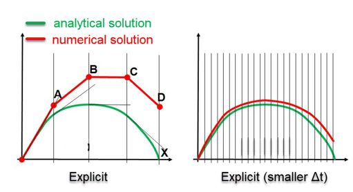
Figure 17: The effect of increment size on the results for Explicit solvers [1].
6.1.1 Automatic Time Incrementation
Abaqus Explicit uses an approximated method to ensure that the solution remains stable. This is achieved by setting the maximum increment size to be less than the stable time increment. There are two options for automatically calculating the stable time increment in the Explicit: “global” estimation and “element-by-element” estimation.
The element-by-element method limits the maximum increment size to the constant value in Equation (1).
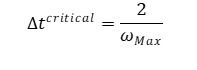 |
(1) |
Where ωmax is the largest frequency in the model. The Explicit calculates the frequency for each element based on the material properties and the element size. The below figure provides instructions on how to select the “Element-by-element method” in the “Edit Step” window in Abaqus.
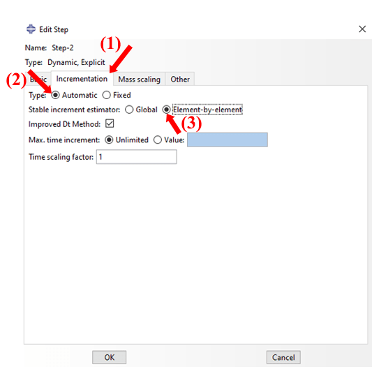
Figure 18: Choosing the Element-by-element method in the Abaqus “Edit Step” window.
The element-by-element method does not consider the effects of boundary conditions and contacts, during the solution, on the maximum increment size. This may lead to unnecessarily large increment sizes and inefficient analysis.
To overcome the limitation of the element-by-element method in updating the model’s frequency, Abaqus Explicit offers the global estimation option. Global estimation updates the maximum increment size based on the real-time state of the model. This allows for larger time increments compared to the element-by-element method, making it more computationally efficient. The Explicit employs the global estimation method by default.
6.1.2 Fixed Time Incrementation
In some scenarios, the analysis requires an accurate representation of higher-mode responses. For such cases, the user must specify a smaller increment size relative to the element-by-element or global methods. This is where the fixed method becomes valuable. The below figure shows how to define a fixed increment size in an Explicit step.
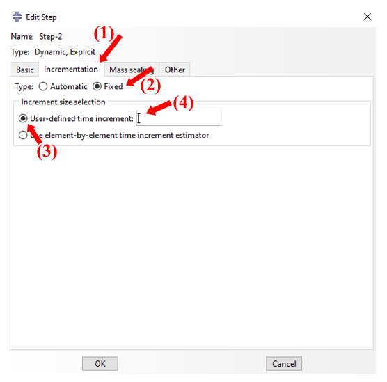
Figure 19: Choosing the Fixed method in the Abaqus “Edit step” window.
It is important to note that when using a fixed increment size, Abaqus does not check the stability condition. So, it is crucial to carefully select a fixed increment size that guarantees stable results.
6.2 The Maximum Increment Size in Abaqus Standard
In the Standard solver, unlike the Explicit solver, convergence must be checked at each increment. Therefore, we are less likely to experience instability issues related to the increment size. You can employ significantly larger increment sizes, without limitations, in Implicit vs Explicit solvers. Moreover, the Standard solver can automatically reduce the defined increment size to prevent converge issues. However, you must be careful not to choose an increment size that is too large. In this situation, Abaqus breaks the increments repeatedly due to convergence issues. This negatively affects the computational cost.
According to the below figure, the Abaqus Standard’s increment size has no significant impact on the analysis results. So, the Standard solver is a more reliable choice compared to the Explicit solver. However, achieving convergence within an increment may require numerous iterations or may not always occur. This highlights a significant limitation of Implicit vs Explicit solvers.
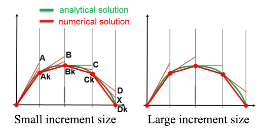
Figure 20: The effect of increment size on the results for Abaqus Standard solver [1]
Note: Monitoring energy balance in Abaqus/Explicit is essential for verifying simulation accuracy, especially in dynamic analyses involving impacts or complex contacts. The solver calculates various energy components—such as internal energy (ALLIE), kinetic energy (ALLKE), and external work (ALLWK) to ensure the total energy (ETOTAL) remains nearly constant throughout the simulation. Significant deviations in ETOTAL can indicate issues like excessive artificial strain energy or unstable contact interactions.
For example, in a quasi-static uniaxial tensile test using Abaqus/Explicit, the kinetic energy should remain below 5–10% of the internal energy. If the kinetic energy exceeds this threshold, it may suggest that the simulation is not truly quasi-static, potentially necessitating a switch to Abaqus/Standard for better stability.
Conversely, in simulations with high-speed impacts or severe contact nonlinearities, Abaqus/Explicit is often more suitable due to its robust handling of such complexities. However, careful monitoring of energy components is still crucial. For instance, excessive artificial strain energy might indicate mesh issues, while a significant increase in ETOTAL could point to numerical instabilities.
By analyzing energy outputs, engineers can make informed decisions about solver selection and model adjustments, ensuring accurate and reliable simulation results.
7. Conclusion: Pick Smart, Simulate Smarter
When it comes to Abaqus Standard vs Explicit, there’s no one-size-fits-all answer. Both solvers are powerful—but they shine in different scenarios.
Use Abaqus Standard (also known as Abaqus Implicit) when you’re working with stable, slow, or linear problems that benefit from accuracy and efficiency. Go for Abaqus Explicit (or Abaqus Dynamic Explicit) when things get fast, nonlinear, or messy—like crashes, impacts, or complex contact.
Still unsure? Start small. Run both solvers on a simplified model. Compare run time, stability, and results. That little experiment can save hours—or even days—later on.
The key isn’t just picking the right solver. It’s knowing why you picked it.
Now that you understand how Abaqus Implicit vs Explicit works under the hood, you’re in a much better place to make that choice with confidence.
In the video below, prepared by our team, see the complete comparison between the Standard solver and the Explicit solver:
Until now, we have tried to explain ‘Abaqus Standard and Explicit’ thoroughly so that you can choose the right solver for your needs. Here, you can find Abaqus Examples for training and understand the concept of these solvers and how to use each one properly.
additionally, It would be useful to see Abaqus Documentation to understand how it would be hard to start an Abaqus simulation without any Abaqus tutorial. Also, please share your views with the CAE Assistant experts in the comment section. We really appreciate your feedback, as it helps us improve our tutorials and fulfill all your CAE needs without requiring additional tutorials.
 |
⭐⭐⭐Free Abaqus Course | ⏰10 hours Video 👩🎓+1000 Students ♾️ Lifetime Access
✅ Module by Module Training ✅ Standard/Explicit Analyses Tutorial ✅ Subroutines (UMAT) Training … ✅ Python Scripting Lesson & Examples |
You can have the PDF of this post by clicking on CAE Assistant- Abaqus implicit or Abaqus explicit
Which of the Explicit or Standard solvers is more suitable for my problem?
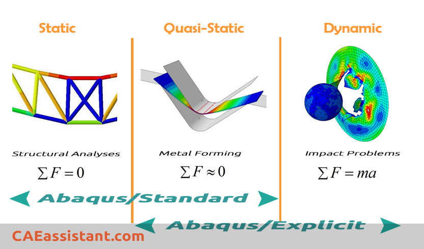
Abaqus/Standard is a good choice to solve static, low-speed dynamic, steady-state transport, or smooth nonlinear analyses. On the other hand, Abaqus/Explicit is the clear choice for quasi-static events such as the rolling of hot metal, severely nonlinear behavior such as contact, transient response, or high-speed dynamic analyses such as crash analysis or drop test. There are, however, certain problems that can be simulated well with either program.
What are the main differences between Explicit and Implicit Solvers in Abaqus?
- Implicit is unconditionally stable.
- Implicit schema is incremental as well as iterative. However, the explicit schema is only incremental.
- In terms of cost per increment, it is costly for implicit and cheaper for explicit.
- Disk space and memory usage are typically much smaller than that implicit: look at this diagram.
What is the difference between the solving strategy of Abaqus/Standard and Abaqus/Explicit?
These solvers are based on two approaches in FEM analysis, namely implicit (for Abaqus/Standard) and explicit. The distinction between the two different numerical approaches makes it possible to understand which solver to use. Abaqus/Standard must iterate to determine the solution to a nonlinear problem, but Abaqus/Explicit determines the solution without iterating by explicitly advancing the kinematic state from the previous increment.
What methods are used to analyze problems in Implicit and Explicit Solver?
In the case of the implicit method, equilibrium is enforced between externally applied load and internally generated reaction forces at every solution step (Newton Raphson method).
In the case of the explicit method, there is no enforcement of equilibrium. But this does not mean that explicit is not accurate. You can minimize its deviation from equilibrium to almost zero by increasing the number of solution steps, i.e. reducing the time step size.
How can we solve problems that involve several analysis stages?
Abaqus provides a useful capability for simulations involving several analysis stages. In this ability, the user can start a simulation in Abaqus/Explicit. Then the results at any point within the solver run can be transferred as the starting point for continuation in Abaqus/Standard. The user will define new model information during the import analysis.
Thank you for being with us in this article. In order to always provide you with up-to-date and engaging content, we need to be familiar with your educational and professional experiences so that we can offer articles and lessons that are most useful to you.
Good write-up. I definitely appreciate this site. Keep it up! Elle Tanny Kirtley
Wow, superb blog layout! How long have you been blogging for? you make blogging look easy. The overall look of your website is excellent, as well as the content! Jacquelynn Kareem Ardyth
Hello, thank you for this article. I needed to choose one of these two solver to solve my problem. This article helped me choose the most suitable solver. thank you