
All about Abaqus Material Models

Choosing the right material model in Abaqus is essential for ensuring accurate and reliable finite element analysis (FEA). The material model selected directly impacts the simulation’s performance, affecting its ability to predict real-world behaviors such as elasticity, plasticity, or failure. Many engineers struggle with finding the right model for their specific use case, as Abaqus offers a variety of options to describe different material behaviors (Abaqus Material Models).
This blog discusses making informed choices when selecting a material model in Abaqus. It covers the main types of Abaqus material models, such as elastic and inelastic models, complex viscoelastic material behaviors, and the definition of damage types. Knowing when to use a linear or Abaqus nonlinear material model is critical, and the guide explains how different models are appropriate for specific materials such as metals, polymers, and composites under various loading conditions. It will also include the most important strategies for defining and using linear and non-linear materials.
The material library in Abaqus is intended to provide comprehensive coverage of both linear and nonlinear, isotropic and anisotropic material behaviors. Some of the mechanical behaviors offered are mutually exclusive: such behaviors cannot appear together in a single material definition. Some behaviors require the presence of other behaviors; for example, plasticity requires linear elasticity. Throughout the blog, you’ll learn how to approach material modeling in Abaqus, including understanding the behavior of elastic and plastic materials, handling time-dependent properties like viscoelasticity, and even simulating progressive damage. By the end, you’ll have a clear understanding of the types of models available, when to use them, and how to improve the accuracy of your simulations with advanced techniques.

1. The Difference Between Linear and Non-linear Materials
In finite element analysis (FEA), understanding the distinction between linear and nonlinear materials is crucial. It helps ensure accurate simulations and proper model selection in Abaqus material models. This context explains the key differences and how Abaqus handles both material types.
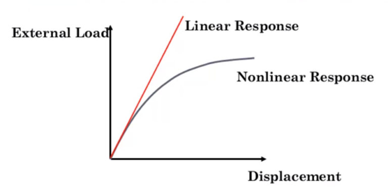
Figure 1: The difference between linear and non-linear behavior of materials [Ref]

|

|
|
1.1. Linear Materials
In Linear Analysis, when we load a structure (like with a force or pressure), the displacement (how much the structure moves) is directly proportional to the load.
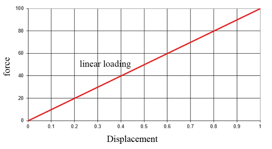
Figure 2: Linear Behavior
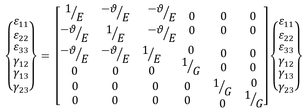
These models are suitable for small deformations and stress scenarios where material behavior remains predictable and reversible. The simplest form of linear elasticity is the isotropic case, and the stress-strain relationship is given by:
The elastic properties are completely defined by giving Young’s modulus, E, and Poisson’s ratio, ![]() . The shear modulus, G, can be expressed in terms of E and as
. The shear modulus, G, can be expressed in terms of E and as ![]() . These parameters can be given as functions of temperature and of other predefined fields, if necessary in Abaqus.
. These parameters can be given as functions of temperature and of other predefined fields, if necessary in Abaqus.
Plane stress is a simplified state of stress within a material where the normal stress and sheer stresses perpendicular to a particular plane (the x-y plane) are assumed to be zero. In other words, the stress components σz, τxz, and τyz are considered negligible. This condition typically arises in thin, flat structures like plates or sheets, where the loads are applied uniformly over the thickness and act within the structure’s plane. The body’s geometry resembles a plate with one dimension (the thickness) significantly smaller than the other.
In plane stress, the stress-strain relationship for isotropic materials is simplified, and the constitutive matrix (or stress/strain matrix) becomes:
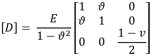
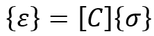
The strain components can be expressed in terms of stress components using the compliance matrix [C], which is the inverse of the stiffness matrix [D].
In the equation above, it is evident that the stress and strain have a linear relationship, indicating the material’s elastic state. This means that in the elastic state, the stress changes in direct proportion to the strain, and the material will return to its original state after being loaded. This principle is also known as the principle of elasticity.
It is important to note that the linear elastic model has limitations. It is only suitable for small strains, typically less than 5%. When dealing with large deformations or plasticity, more complex Abaqus material models like hyperelastic or elastoplastic are necessary. Overall, understanding the characteristics and limitations of the linear elastic model is vital for selecting the appropriate material model and ensuring accurate simulation results in Abaqus.
| If you need deep training, our Abaqus Course offerings have you covered. Visit our Abaqus course today to find the perfect course for your needs and take your Abaqus knowledge to the next level! |
1.2. Nonlinear Materials
The difference between linear and nonlinear materials is an important concept. Linear materials have a predictable relationship between stress and strain, so when force is applied, they stretch proportionally and return to their original shape when released. Many common materials, like steel and rubber, display this behavior within a certain range of stress and strain.
However, a vast array of materials defies this simplicity, exhibiting a non-proportional relationship between stress and strain. These are the nonlinear materials. Picture modeling clay that, once deformed, retains its new shape—a clear demonstration of nonlinearity. This complexity arises from various factors such as plasticity, large deformations, material damage, and time-dependent effects. In essence, nonlinear materials do not follow a predictable, constant ratio between stress and strain, often experiencing permanent deformation and exhibiting path dependence.
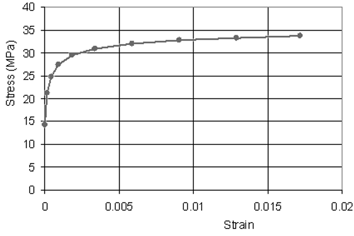
Figure 3: An example of the behavior of plastic material
Metals undergoing plastic deformation, polymers, biological tissues, and soils all fall under the umbrella of nonlinear materials. Understanding their behavior is paramount for engineers and scientists across disciplines. For instance, designing safe and efficient structures necessitates accurate predictions of how materials will respond under diverse loading conditions.
In manufacturing, comprehending nonlinearity helps optimize processes and develop new materials with tailored properties. However, analyzing nonlinear materials is no simple task. Their complex behavior often demands advanced numerical methods like finite element analysis (FEA) to solve governing equations and capture the material’s response. These simulations, though computationally intensive, provide valuable insights into material behavior under various loads, enabling informed decisions regarding material selection, design, and performance optimization.
Abaqus has an extensive library of built-in material models that cover various nonlinear phenomena. These include hyperelasticity for large elastic deformations, plasticity for permanent deformation, viscoelasticity for time-dependent behavior, creep, damage, and failure. Additionally, the software allows users to implement their own Abaqus material models through subroutines, catering to specialized or advanced material responses.
In addition to Abaqus material models, Abaqus offers a range of analysis procedures to handle nonlinearity. Static analysis is used for problems where loads are applied gradually and with negligible inertia effects, while dynamic analysis tackles nonlinear dynamic problems considering inertia and damping effects. For highly nonlinear and transient scenarios, explicit dynamics are employed to handle large deformations, contact, and material failure with precision.
The software also offers various element types including solid elements for three-dimensional structures, shell elements for thin-walled structures, and beam and truss elements for slender structures. Furthermore, Abaqus excels in managing complex contact and interaction scenarios that frequently arise in nonlinear problems, such as contact between deformable bodies, self-contact, and friction.
In conclusion, linear and nonlinear Abaqus material models represent two distinct classes of material behavior. While linear materials offer simplicity and predictability, nonlinear materials present challenges and complexities. Nonetheless, the latter are ubiquitous in both engineering and natural systems, offering vast opportunities for innovation and optimization. By mastering the art of modeling and understanding nonlinear materials, engineers and scientists pave the way for advancements in fields ranging from aerospace and automotive engineering to biomechanics and geotechnical engineering.

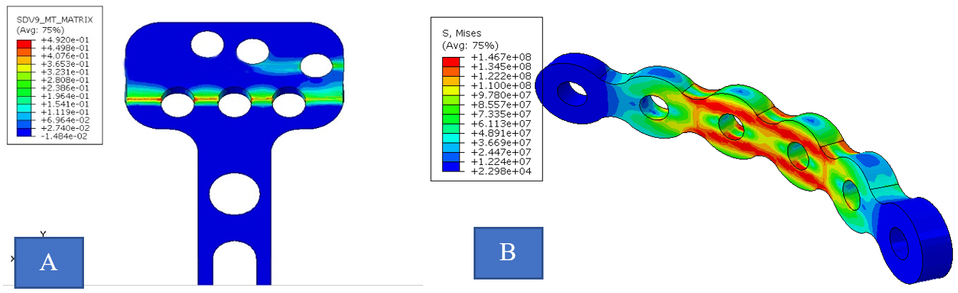
Figure 4: An example of the use of plastic in Abaqus: image A: the damage analysis and the beginning of the rupture of the object and image B: the stress analysis of a piece
As observed, first, we establish the fundamental concept of the behavior of materials under stress and strain and distinguish between materials that exhibit a proportional response (linear) and materials that do not (linear). This understanding enters directly into the second section, which addresses the diverse range of models used to simulate and predict the behavior of various materials in engineering and scientific applications. This relationship lies in choosing appropriate Abaqus material models based on whether the desired materials have linear or non-linear characteristics. Ensures accurate and reliable simulations and analyses. In the second part, we will use these features to briefly explore how to use this category of problems in the Abaqus software.
2. All Kinds of Abaqus Material Models
Understanding the different types of Abaqus material models is the first step toward selecting the right one for your project. Abaqus offers a wide variety of models to represent different mechanical behaviors of In this section, we will discuss elastic, plastic, viscoelastic, and J2 Plastic models and briefly discuss how to use them in Abaqus software. After that, we will do a brief review of progressive damage models to examine how the crack grows and damages it, and finally, we will examine some important strategies for better Abaqus Material Modeling.
2.1. Elastic Mechanical Models
Elastic models describe materials that return to their original shape after being deformed. In Abaqus, linear elasticity is often used when the deformation is small, and the material behavior remains within its elastic limit. This type of behavior is commonly seen in metals, ceramics, and many polymers under low-stress conditions. This type of model is ideal for metals under small stresses and strains, where no permanent deformation occurs.
To define a linear elastic Abaqus material models, users need to specify its properties, including Young’s modulus, Poisson’s ratio, and (If the dynamic solver is used to answer the problem), in the Property module. Additional properties such as thermal expansion coefficient or damping coefficients may be required depending on the analysis type and material behavior.
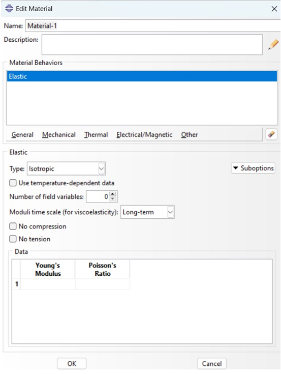
Figure 5: Define linear material in Abaqus
2.2. Plastic and Inelastic Mechanical Abaqus Material Models
Plastic deformation occurs when a material is stressed beyond its yield point, the threshold where it transitions from elastic to plastic behavior. Before this point, the material deforms elastically (recoverably). Once it crosses the yield point, permanent (plastic) deformations occur. Yield stress is a critical parameter in material mechanics that defines the stress level at which a material begins to undergo plastic deformation.
The critical point where a material transition from elastic to plastic deformation is typically measured in units of pressure like Pascals or psi. This pivotal point, the yield point, is where the stress-strain relationship deviates from linearity. Importantly, the yield stress is material-dependent, with materials like steel exhibiting high yield stress values, while aluminum and polymers have lower values.
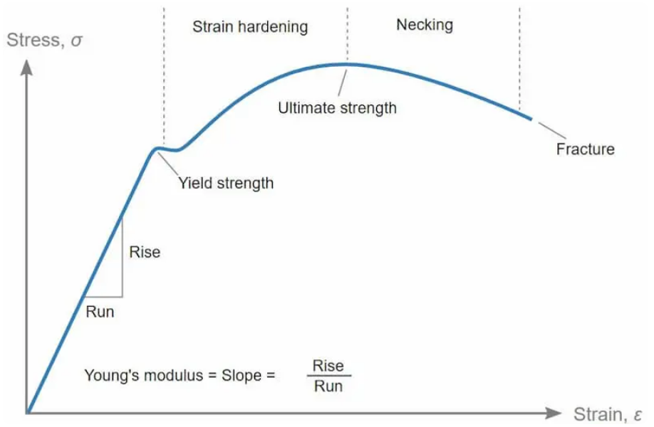
Figure 6: Showing the behavior of a material elastic-plastic based on stress and strain [Ref]
Abaqus material models provide several Abaqus plasticity models that can be used depending on the material behavior and loading conditions. These include the classical metal plasticity model, creep model, viscoplasticity, and more specialized models for complex behaviors like ductile damage and progressive failure.
2.3. J2 Plasticity Model
The classical J2 plasticity model is the most commonly used plastic model in Abaqus, suitable for metals under moderate plastic deformation. It is based on the von Mises yield criterion, which assumes that yielding occurs when the second invariant of the deviatoric stress tensor reaches a critical value (the yield stress). This behavior is governed by the flow rule and hardening laws. The material yields when the von Mises stress, ![]() , exceeds the yield stress
, exceeds the yield stress ![]() :
:
![]()
The von Mises stress is calculated as:
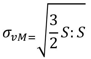
Where S is the deviatoric stress tensor.
In the context of the J2 plasticity model, the associated flow rule defines how the plastic strain develops in a material once it starts to yield. It essentially states that the direction of plastic flow aligns with the normal to the yield surface at the current stress point.
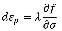
Where λ is a plastic multiplier, determining the rate at which plastic deformation progresses.
Hardening laws dictate how a material strengthens as it is subjected to plastic deformation and its internal structure changes, which can lead to an increase in strength. This phenomenon is crucial for engineers and designers to understand, as it affects the performance and safety of structures and components.
Types of Hardening Laws
- Isotropic Hardening: This law assumes that the yield surface expands uniformly in all directions as the material is deformed. It means that the material’s yield strength increases equally regardless of the direction of the applied stress.
- Kinematic Hardening: Unlike isotropic hardening, kinematic hardening allows the yield surface to translate in stress space. This means that the material can exhibit different yield strengths depending on the direction of loading, which is particularly useful for materials that experience cyclic loading.
- Nonlinear Hardening: Many materials do not follow a simple linear relationship between stress and strain. Abaqus Nonlinear material hardening laws account for more complex behaviors, where the rate of hardening changes as the material undergoes deformation. This is often modeled using parameters that are determined experimentally.
In Abaqus material models, to use the plastic behavior for the material, it is very important to know the material’s behavior and hardening. Therefore, as shown in the figure below, the amount of stress and strain in the non-linear region must be entered in the data section, and the hardening method will also be specified in the hardening shutter.
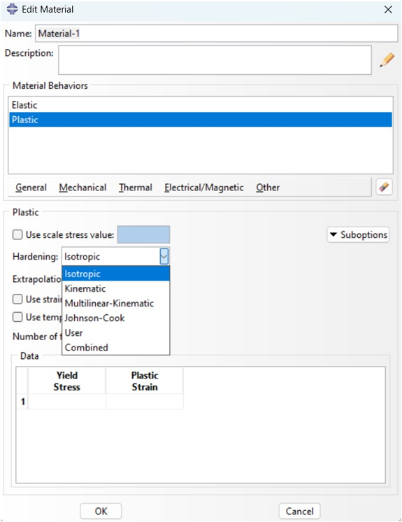
Figure 7: How to apply J2 theory in Abaqus
2.4. Viscoelasticity
The concept of viscosity refers to a fluid’s ability to resist flowing. A fluid with high viscosity resists movement, while one with low viscosity flows easily. For instance, water has a low viscosity and flows more freely compared to syrup, which has a high viscosity. Viscoelastic material models capture the time-dependent behavior of materials that exhibit both elastic and viscous responses.
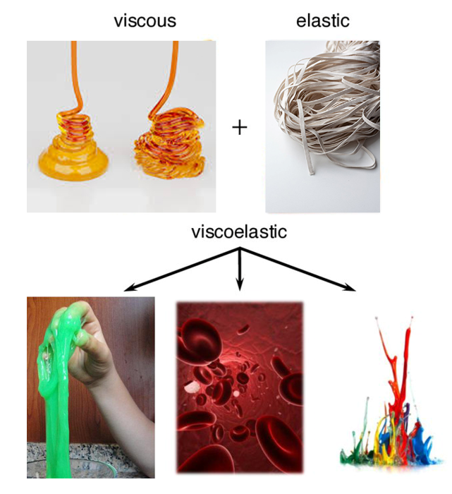
Figure 8: viscoelastic material, showcasing both its elastic and viscous properties
These models are crucial for simulating polymers, rubbers, and biological tissues, where the material’s behavior changes depending on the duration and rate of loading.
In linear viscoelastic materials, the relationship between the material’s response (As you know, one of the most common results is viscoelastic creep) and the applied load (stress) can be expressed as separate functions. This separation allows for simpler mathematical modeling. Essentially, all linear viscoelastic behavior can be described using a Volterra equation, which establishes a connection between stress and strain in the material over time.
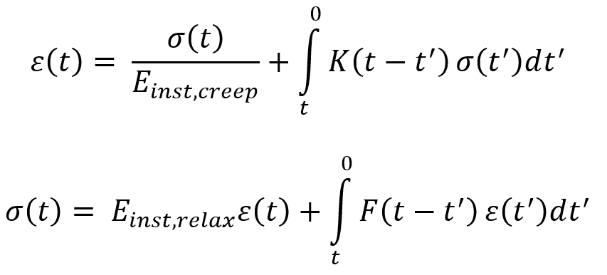
Where:
t is time , σ(t) is stress , ε(t) is strain, Einst,creep and Einst,relax are instantaneous elastic moduli for creep and relaxation , K(t) is the creep function, and F(t) is the relaxation function. Linear viscoelasticity is usually applicable only for small deformations. Nonlinear viscoelasticity is when the function is not separable. It usually happens when the deformations are large or if the material changes its properties under deformations. An anelastic material is a special case of a viscoelastic material: an anelastic material will NOT fully recover to its original state on the removal of load. Viscoelastic materials are used in various applications, including:
- Shock Absorption: Their ability to dissipate energy makes them ideal for shock absorbers and vibration dampers.
- Biomedical Implants: They are used in artificial joints and tissue engineering scaffolds due to their biocompatibility and ability to mimic natural tissues.
- Adhesives and Sealants: They provide strong and durable bonds due to their viscoelastic properties.
- Food Processing: The viscoelastic behavior of food materials is crucial in understanding their texture and processing.
Are you interested in learning how to effectively model viscoelastic materials in Abaqus? If so, you’ve come to the right place! Let’s dive into the essential steps for modeling viscoelastic materials in Abaqus.
When dealing with viscoelastic materials in Abaqus, it’s crucial to define their properties accurately. In the time domain, you can use the Prony series representation to specify the shear or bulk relaxation moduli along with their corresponding relaxation times, as shown in figure(a) below. If you have frequency-dependent data, Abaqus allows you to input the storage and loss moduli as a function of frequency as shown in the figure(b) below.
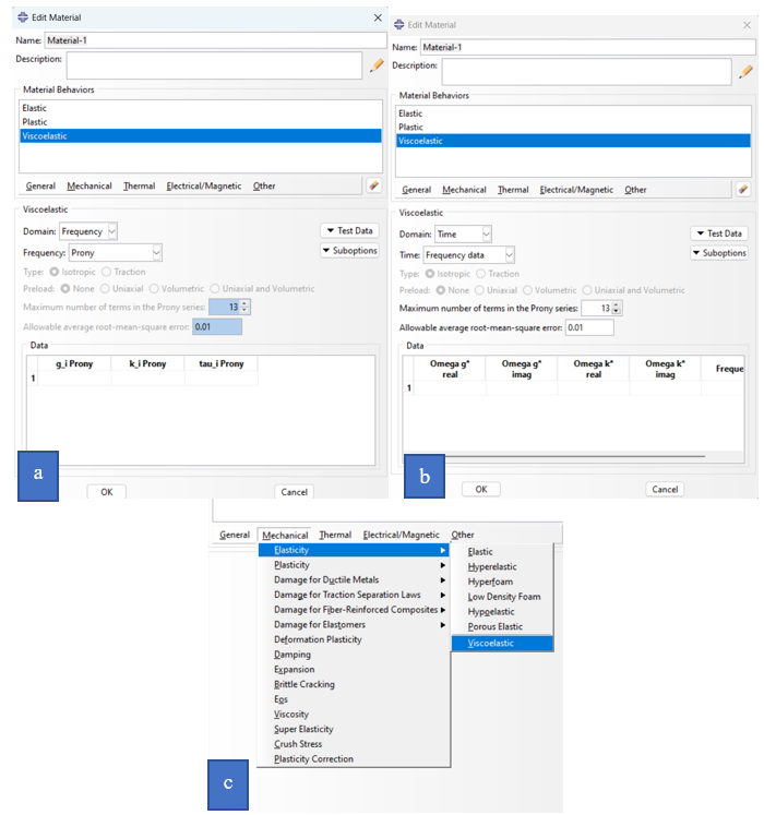
Figure 9: a) use the Prony series representation to specify the shear or bulk relaxation moduli along with their corresponding relaxation times, b) the Prony series representation to frequency-dependent data, c) the menu of viscoelastic
- In figure a: g_i, k_i, and tau_i are the constants of the Prony series.
- In figure b: the real part of g and the imaginary part of g are used.
- The Value of a is the Real part of k. If the material is incompressible, this value is ignored. The imaginary part of k If the material is incompressible, this value is ignored.
- Value of b: If the material is incompressible, this value is ignored.
3. A Complete Guide to Abaqus Material Models Definition
Some of the mechanical behaviors offered are mutually exclusive: such behaviors cannot appear together in a single material definition. Some behaviors require the presence of other behaviors; for example, plasticity requires linear elasticity.
A material definition (Abaqus Material Models Definition) can include behaviors that are not meaningful for the elements or analysis in which the material is being used. Such behaviors will be ignored. For example, a material definition can include heat transfer properties (conductivity, specific heat) as well as stress-strain properties (elastic moduli, yield stress, etc.). When this material definition is used with uncoupled stress/displacement elements, the heat transfer properties are ignored by Abaqus; when it is used with heat transfer elements, the mechanical strength properties are ignored. This capability allows you to develop complete material definitions and use them in any analysis.
There are no general restrictions on the use of particular material behaviors with solid, shell, and beam elements. Any combination that makes sense is acceptable. However, there may be some exceptions.
Any number of materials can be defined in an analysis. Each material definition can contain any number of material behaviors, as required, to specify the complete material behavior. For example, in a linear static stress analysis, only elastic material behavior may be needed, while in a more complicated analysis, several material behaviors may be required.
A name must be assigned to each material definition. This name allows the material to be referenced from the section definitions used to assign this material to regions in the model.
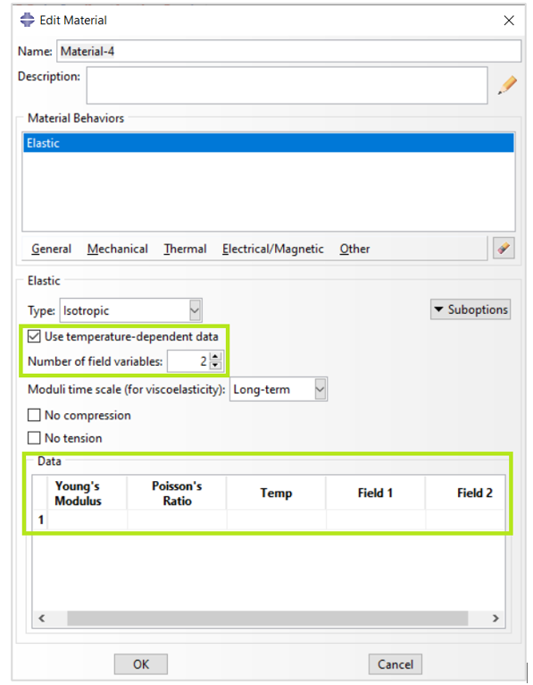
Figure 10: Material definition in Abaqus/CAE
Material properties can be defined as simple constant values or they can be dependent on variables such as temperature or field variables. (Abaqus Material Models Definition)
Material data are often specified as functions of independent variables such as temperature. Material properties are made temperature-dependent by specifying them at several different temperatures. In some cases, a material property can be defined as a function of variables calculated by Abaqus; for example, to define a work-hardening curve, stress must be given as a function of equivalent plastic strain.
In Abaqus material models, material properties can also be dependent on “field variables” (user-defined variables that can represent any independent quantity and are defined at the nodes, as functions of time). For example, material moduli can be functions of weave density in a composite or of phase fraction in an alloy. The initial values of field variables are given as initial conditions and can be modified as functions of time during an analysis. This capability is useful if, for example, material properties change with time because of irradiation or some other precalculated environmental effect.
For example, in figure 11, the elastic material properties are chosen to be both temperature and field variable-dependent.
Figure 11: Material properties dependence on temperature and field variables
3.1. Interpolation of Material Data
In the simplest case of a constant property, only the constant value is entered. When the material data are functions of only one variable, the data must be given in order of increasing values of the independent variable. Abaqus then interpolates linearly for values between those given. (Abaqus Material Models Definition)
The property is assumed to be constant outside the range of independent variables given. Thus, you can give as many or as few input values as are necessary for the material model. If the material data depends on the independent variable in a strongly nonlinear manner, you must specify enough data points so that linear interpolation captures the nonlinear behavior accurately.
In Abaqus material models when material properties depend on several variables, the variation of the properties with respect to the first variable must be given at fixed values of the other variables, in ascending values of the second variable, then of the third variable, and so on. The data must always be ordered so that the independent variables are given increasing values. This process ensures that the value of the material property is completely and uniquely defined at any values of the independent variables upon which the property depends (Figure 12).
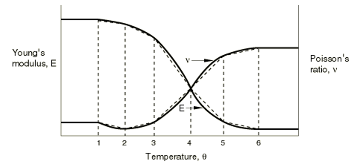
Figure 12: The material Young’s modulus and the Poisson’s ratio as functions of temperature
For temperatures that are outside the range defined by ![]() and
and ![]() , Abaqus assumes constant values for
, Abaqus assumes constant values for ![]() and
and ![]() . The dotted lines on the graph represent the straight-line approximations that will be used for this model.
. The dotted lines on the graph represent the straight-line approximations that will be used for this model.
4. Change Material Properties Between Steps in Abaqus
In some analyses, you may have to change Abaqus material models properties between steps due to various reasons such as:
- Phase transitions
Material properties can change during phase transitions, such as melting or solidification, and should be accounted for in the simulation.
- Temperature-dependent properties
Material properties can vary with temperature, leading to the need for property updates during thermal loading steps.
- Dynamic behavior:
The material properties of some materials, such as rubber or foam, can change under high-speed loading or large deformations.
- Time-dependent properties
Some materials exhibit time-dependent behavior, such as creep and relaxation, requiring property updates over time.
Some of the mentioned reasons can be satisfied by the default options that Abaqus has provided like temperature-dependent properties as discussed earlier or creep phenomenon simulation; but for some of the material changes the analyst must decide how to implement the material behavior transition in the analysis. (Abaqus Material Models Definition)
In the case of changing material at a special moment during your analysis, it is more convenient to include this material change in the material properties as much as possible. For example, in the case of damage and material degradation, there are several models that predict the onset and progression of damage in Abaqus. You can also use the “User Subroutine” to implement your own damage model in the analysis.
However, sometimes you may want to change the material from material No.1 to material No.2 at a specific condition in your model (e.g., these materials differ in the density values) which are already defined in the material section in the ‘Property’ module. One way to achieve this is to use solution-dependent variables and using a user subroutine. By defining these variables, you can link material properties to the values of these variables.
4.1. Specifying Material Data as Functions of Solution-Dependent Variables
In Abaqus, you can introduce dependence on solution variables with a user subroutine. User subroutines “USDFLD” in Abaqus/Standard and “VUSDFLD” in Abaqus/Explicit allow you to define field variables at a material point as functions of time, of material directions, and of any of the available material point quantities.
User subroutines “USDFLD” and “VUSDFLD” are called at each material point for which the material definition includes a reference to the user subroutine.
These subroutines can be used to introduce solution-dependent material properties since such properties can easily be defined as functions of field variables. They will be called at all material points of elements for which the material definition includes user-defined field variables.
Abaqus USDFLD and VSDFLD have a very broad scope, and in general, you can use these two subroutines whenever you have a parameter in the software material environment that you want to rely on another variable.
If you have a complete characterization of your material behavior, you can use the “UMAT” subroutine instead. This advanced method allows you to write custom subroutines to define complex material behavior and changes.
User subroutine “UMAT” can be used to define the mechanical constitutive behavior of a material. It will be called at all material calculation points of elements for which the material definition includes a user-defined material behavior and can be used with any procedure that includes mechanical behavior. UMAT can use solution-dependent state variables. It also can be used in conjunction with user subroutine USDFLD to redefine any field variables before they are passed in.
By using the mentioned ways, you can change material at steps in your analysis. There may be some other ways too. Abaqus has a diverse world of options which enables you to use one or a combination of them to make your analysis more and more realistic and accurate. Remember to carefully consider the types of changes, appropriate methods, and validation steps to ensure your simulations reflect real-world scenarios.
5. Modeling Progressive Damage
In many cases, materials experience damage or failure over time due to repeated loading or extreme conditions. Progressive damage in Abaqus Material models simulate how cracks or fractures evolve in a material, which is essential for fatigue analysis or understanding failure mechanisms in structures. You can learn more about damage in this blog: “Ductile Damage: A Comprehensive Study on Failure Mechanisms of Ductile Materials”
Explore our comprehensive Abaqus tutorial page, featuring free PDF guides and detailed videos for all skill levels. Discover both free and premium packages, along with essential information to master Abaqus efficiently. Start your journey with our Abaqus tutorial now!
The CAE Assistant is committed to addressing all your CAE needs, and your feedback greatly assists us in achieving this goal. If you have any questions or encounter complications, please feel free to share it with us through our social media accounts including WhatsApp.
6. Conclusion
The article focuses on the critical task of selecting the right material model in Abaqus to ensure accurate finite element analysis (FEA). Abaqus Material models play a vital role in determining how well simulations predict real-world behaviors such as elasticity, plasticity, and failure. Given the diversity of materials and loading conditions encountered in engineering, choosing the appropriate model is essential for reliable analysis and simulation outcomes.
It begins by distinguishing between linear and nonlinear materials, explaining how linear materials exhibit predictable behavior while nonlinear materials, such as those undergoing plastic deformation or large deformations, require more complex models. This is followed by a discussion of various material models in Abaqus, including elastic, plastic, viscoelastic, and progressive damage models. These models are important for accurately representing the behavior of metals, polymers, composites, and biological tissues under different stress conditions.
The article also explores hydrodynamic models, which simulate fluid-like behavior in extreme conditions such as explosions or underwater impacts. Furthermore, strategies for improving the accuracy of material simulations are presented. These include using high-quality experimental data, performing mesh refinement, and validating the model against real-world data to ensure reliable simulation results.
In conclusion, the article highlights the importance of understanding material behaviors and selecting appropriate models in Abaqus for accurate simulations. By applying advanced techniques to enhance simulation accuracy, users can achieve more reliable and meaningful outcomes in their engineering analyses.