


Introduction to Creep | Creep Abaqus modeling
One of the important issues in studying mechanical systems is determining the service life of their components. Engineers need to be aware of the time to failure of system components to prevent extensive damages. As you may know, one of the causes of mechanical component failure is the creep phenomenon.
Creep is a phenomenon in materials science and engineering where gradual deformation or strain occurs over time under a constant load or stress, particularly at elevated temperatures. Understanding and analyzing creep behavior is of significant importance in various industries, including power generation, aerospace, and manufacturing. Creep analysis allows engineers to predict the long-term deformation and potential failure of materials, enabling the design of structures and components that can withstand these conditions. Therefore, determining the life of components subjected to creep is of great importance.
Lesson 1: What is Creep?
In this lesson, first, the creep phenomenon is defined: Creep is time-dependent deformation of a material, and it typically occurs at high temperatures and under constant stress. These stresses are usually lower than the yield stress. Therefore, we can consider three influential factors on creep: time, temperature, and stress level. Since many industrial components operate under constant stress lower than the yield stress and in high-temperature environments, numerous industrial components experience failure due to creep phenomenon. Therefore, the investigation and simulation of the creep phenomenon are of great importance.
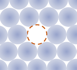
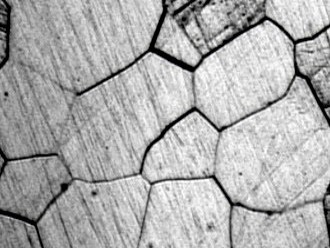
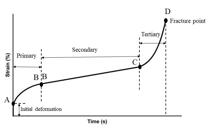
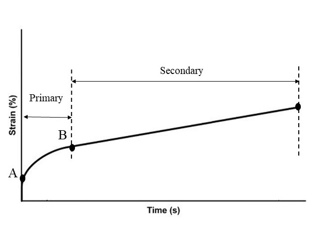
Moreover, you will learn more about the temperature factor: The first temperature effect is Vacancy Concentration. In crystalline materials, some atoms are missing from their intended positions in the lattice. These defects in the crystal lattice are called vacancy Concentration. Increasing temperature leads to an increase in the concentration of vacancies, and an increased concentration of vacancies aids the creep process. Also, the creep curve will be discussed, which helps you to better understand the stages of creep. Usually, the strain-time diagram is used to study the creep process. To examine this diagram, you should know the standard creep test methods. The standard creep test is generally performed in two ways: constant load and constant stress. In first method, only a constant load is applied to the sample and the amount of load does not change over time. In the second method, which requires advanced equipment, a constant stress is applied. In this method, considering that the cross-sectional area of the sample is constantly decreasing during the test, the force must also decrease in order to keep the stress constant.
Lesson 2: What are creep life estimation models?
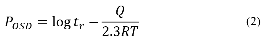
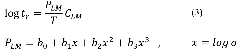
Engineers need to be aware of the time to failure of system components to prevent extensive damages. As you may know, one of the causes of mechanical component failure is the creep phenomenon. In this section, you will study methods for determining the life of components under creep: Larson-Miller, Orr-Sherby-Dorn, and Polynomials estimation models.
Lesson 3: What are creep models?
There are several models to simulate the creep behavior with and in this lesson, you will learn all the models in the Abaqus. Simulation of creep behavior in Abaqus, provides valuable insights into material response under sustained loads and high temperatures. Abaqus offers sophisticated creep modeling capabilities that enable engineers to accurately predict creep deformation and assess the structural integrity of components over time. In Abaqus, creep can be simulated using various creep models:
- Time-Hardening law: When dealing with loading conditions where the stress or temperature is changing, it is necessary to have a proper hardening relation to accurately models the material behavior. However, in general, it is not recommended to use the time hardening relation when the stress is changing.
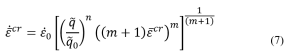
- Time-Power law: The time-power law is equivalent to the time hardening law but with modifications to avoid computational problems.
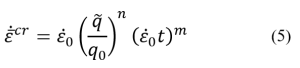
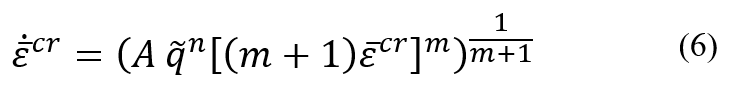
- Strain-Hardening law: This law is suitable for modeling the creep behavior under changing stress conditions. However, similar to the time hardening law, it is more appropriate for low stress levels.
- Power law: The power law is equivalent to the strain hardening law with some slight differences.
- Hyperbolic-Sine law: The hyperbolic sine law, along with the subsequent laws, effectively models creep due to their consideration of the effects of temperature, stress, and time.
- Anand law
- Darveaux law
- Double Power law
These models capture the time-dependent behavior of materials by incorporating parameters like creep exponent, activation energy, and reference stress. Also, if you need another model or a user-defined creep model, you can use the Creep subroutine, which will be explained in workshop 2. Moreover, according to the Abaqus documentation, none of the above models are suitable for modeling the creep cyclic loading, which leaves us with only one option and that is the Creep subroutine.
Workshop 1: Creep process on a standard specimen using Strain-Hardening law
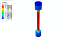
In this workshop, the creep process is simulated to a standard specimen using the Strain-Hardening law. One side of the model is fixed and the other is subjected to the tensile stress. Two steps are used for this modeling; one for the initial loading and the other for the creep. The first step is “Static, General” and the second step is “Visco”. The “Visco” step is for quasi-static problems and the ones whose answers are time-dependent, such as creep and viscoelasticity. In the end, we monitor the strain results due to the creep process.
Workshop 2: Applying creep process on a standard specimen using Creep subroutine
The problem description of this workshop is just like the previous one, but this time the Creep subroutine is used to apply the Strain-Hardening law to the model. The subroutine and all its variables are introduced; the subroutine is explained line by line in this workshop so you can understand how to work with it. In the end, the results of this modeling will be compared with the previous workshop to validate the subroutine results.
It would be helpful to see Abaqus Documentation to understand how it would be hard to start an Abaqus simulation without any Abaqus tutorial. Moreover, if you need to get some info about the FEM, visit this article: “Introduction to Finite Element Method | Finite Element Analysis”. You don’t know which Abaqus software editions are suitable for you, Do not worry! This article would give you info about Abaqus editions: “How to download Abaqus? | Abaqus student & commercial edition” . One note, when you are simulating in Abaqus, be careful with the units of values you insert in Abaqus. Yes! Abaqus don’t have units but the values you enter must have consistent units. You can learn more about the system of units in Abaqus.
Moreover, the general description of how to write a subroutine is available in the article titled “Start Writing a Subroutine in Abaqus: Basics and Recommendations “. If you even do not familiar with the FORTRAN, you can learn the basics via this article: “Abaqus Fortran “Must-Knows” for Writing Subroutines”.


Olga –
I purchased the Creep Analysis in Abaqus training package, and I am extremely satisfied with it. This package provides a comprehensive guide to creep analysis using the Abaqus software. It covers various methods for estimating creep life in system components, such as the Larson-Miller method. . The content is presented clearly and is easy to understand, accompanied by practical examples that demonstrate the best practices for conducting creep simulations. I highly recommend this package to engineers working in the field of creep analysis.
Experts Of CAE Assistant Group –
Thanks for your kind feedback
Fiammetta –
Using this package was truly excellent. Everything was well-explained, and I was able to perform creep analysis effortlessly. The sections on default settings and material definitions were particularly helpful. Do you have any guides for more advanced analyses and detailed explanations on setting creep parameters? I’m looking for more complex analyses, and any additional guidance would be beneficial.
Ginevra –
The tutorial package was very comprehensive and useful. All steps were clearly explained, leaving no ambiguity. I successfully completed the creep analysis and obtained precise results. Can you recommend additional resources for deeper study? I am interested in learning more about the effects of creep in various materials.
Ludovica –
Thank you very much for this excellent package. I was able to perform creep analysis in Abaqus effortlessly. The precise explanations and practical examples were very helpful. Do you plan to release other tutorial packages? I am keen to learn about other areas of mechanical analysis as well.
Ottavia –
This package met all my needs. Thank you for the detailed and complete explanations. The sections on boundary conditions and loading definitions were particularly useful.
Vittoria –
The package was very useful, and I managed to complete my project on time. Your explanations on defining materials and creep parameters were very clear and understandable. Can you provide more guidance on advanced creep parameters and their impact on final results?
Alessio –
Using this package was very easy, and I obtained accurate and reliable results. Your step-by-step guidance was extremely helpful. Do you have plans for hosting educational webinars or online courses? I am interested in participating in more advanced courses.
Bruno –
This package was exactly what I was looking for. Very practical and easy to use. The detailed explanations and practical examples helped me perform creep analysis effortlessly. Can you recommend additional resources for deeper study? I am keen to learn more about advanced mechanical analyses.
Ettore –
I was very satisfied with this package. Everything was well-explained, and I was able to use it easily. The sections on initial settings and boundary conditions were very helpful. Do you have plans to offer other tutorial packages in the future? I am particularly interested in dynamic analyses.
Leandro –
This tutorial package helped me perform creep analysis in Abaqus effortlessly. Your explanations on defining creep parameters and model settings were very precise and clear.
Rinaldo –
Thank you very much for this outstanding package. Everything was well-explained, and I was able to use it easily. The sections on result analysis and output review were particularly helpful. Do you plan to offer more advanced educational courses? I am interested in learning more about creep analysis and material behavior under various conditions.