
Abaqus nonlinear analysis VS linear analysis

The world of FEA engineering thrives on precise simulations that mirror real-world scenarios. But a crucial question often arises: when can a straightforward linear analysis provide sufficient results, and when do we need to navigate the intricate world of nonlinearity? Understanding this fundamental distinction is paramount for choosing the right tools within Abaqus and achieving reliable outcomes (Abaqus nonlinear).
In essence, linear problems exhibit a direct proportionality between cause and effect. Imagine stretching a spring – the force you apply increases steadily with the distance you stretch it. This predictable relationship forms the core of linear analysis. Nonlinear problems, however, challenge this simplicity. Think of bending a metal wire – initially, it bends easily, but as you push further, the resistance increases dramatically. This non-proportional response necessitates the use of nonlinear analysis tools in Abaqus.
This blog post serves as your guide through this critical concept. We’ll delve into the key characteristics of both linear and nonlinear problems, along with the various sources of nonlinearity that FEA engineers encounter routinely. By the end, you’ll be well-equipped to confidently choose the appropriate analysis approach for your Abaqus simulations.
1. What are Linear and Nonlinear problems? | Abaqus nonlinear analysis
In the realm of mechanical engineering, the problems can be categorized into two fundamental types: linear and nonlinear. Understanding the distinction is crucial for choosing the right analytical tools and achieving accurate solutions (Abaqus nonlinear).
Linear problems are characterized by a “direct proportionality” between the input and output. This means that doubling the input always results in a doubling of the output.
Nonlinear problems, on the other hand, exhibit a “non-proportional relationship” between input and output. The response to an input can be complex and unpredictable.
A simple exhibition of linear and nonlinear problems is presented in figure 1. This figure shows the relation between force and displacement of the model for linear and nonlinear problems.
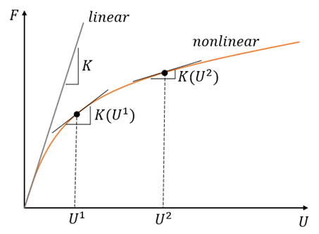
Figure 1: Linear and nonlinear behavior
1.1. Properties of Linear and Nonlinear Problems
Linear problems often exhibit the following key characteristics:
- Existence and Uniqueness: For each load there will be always one and only one solution.
- Superposition: The effect of multiple inputs acting simultaneously is simply the sum of the individual effects of each input.
- Scaling: Scaling the input by a constant factor scales the output by the same factor.
Nonlinear problems exhibit the exact opposite characteristics as what we had for linear problems. Moreover, the solution in nonlinear problems is “History dependent” which means you need to know the loading history to determine the solution.
1.2. Sources of Nonlinearity
There are three common sources of nonlinearity:
1. Geometry
Geometric nonlinearity occurs whenever the magnitude of the displacements affects the response of the structure. May be caused by:
- Large deflections or rotations
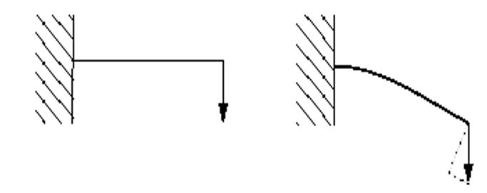
Figure 2: Large deflection of a cantilever beam
- “Snap through”
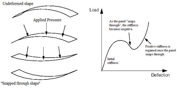
Figure 3: Representation of the behavior of the panel “snaps through”
2. Material
Material nonlinearity occurs when the material response to the applied load deviates from the linear relation between force-displacement or stress-strain.
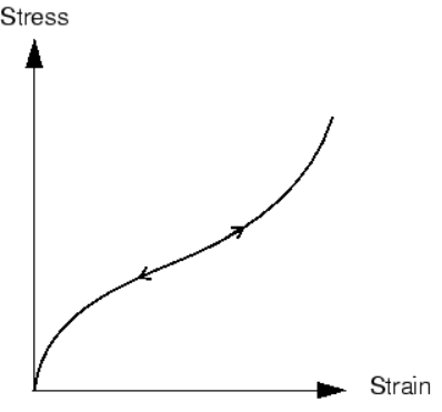
Figure 4: A rubber material response to the applied load
3. Boundary
Boundary nonlinearity occurs if the boundary conditions change during the analysis.
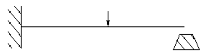
Figure 5: Boundary nonlinearity occurs as the beam tip hits the stop
You can learn more about the nonlinearity resources with practical examples by watching this tutorial: “Abaqus convergence tutorial | Introduction to Nonlinearity and Convergence in ABAQUS”
2. Numerical Techniques for solving nonlinear problems
Numerical techniques approximate solutions using iterative methods that converge to a desired accuracy or meet pre-defined criteria. The choice of a suitable technique depends on the specific problem, available resources, and desired level of accuracy. Two of the common numerical techniques which are also used in Abaqus will be introduced here (Abaqus nonlinear).
2.1. Newton-Raphson Technique
The Newton-Raphson method, named after Isaac Newton and Joseph Raphson, stands as a powerful numerical technique used to find roots of nonlinear equations. It leverages the concept of tangent lines, skillfully employing the function’s first derivative to iteratively refine an initial guess.
The process begins with an initial approximation, denoted as ![]() , which is used to find the equation of the tangent line to the function’s graph at that point. The point where this tangent line intersects the x-axis is then taken as a new approximation,
, which is used to find the equation of the tangent line to the function’s graph at that point. The point where this tangent line intersects the x-axis is then taken as a new approximation, ![]() . This procedure is repeated, iteratively generating a sequence of approximations
. This procedure is repeated, iteratively generating a sequence of approximations ![]() that ideally converge to the function’s root. The method’s effectiveness hinges on the initial guess being sufficiently close to the actual root. A schematic of the Newton-Raphson procedure is shown in figure 6.
that ideally converge to the function’s root. The method’s effectiveness hinges on the initial guess being sufficiently close to the actual root. A schematic of the Newton-Raphson procedure is shown in figure 6.
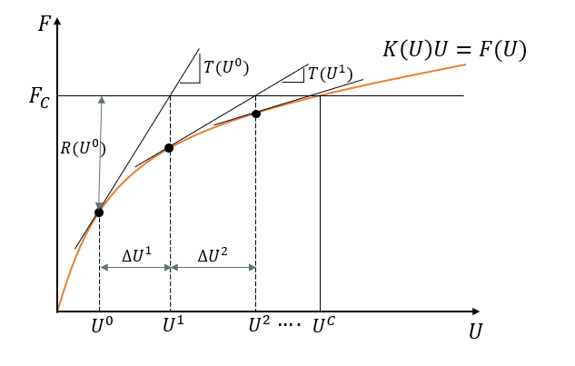
Figure 6: Newton-Raphson procedure to find the converged solution
Newton-Raphson boasts several advantages:
- Fast Convergence: When the initial guess is close to the root, the algorithm converges quickly.
- Wide Applicability: The method works for a wide range of functions, making it versatile.
However, it’s crucial to be aware of its limitations:
- Sensitivity to Initial Guess: Choosing an inaccurate initial guess can lead to divergence or convergence to a different root.
- Derivatives are Essential: The method requires the ability to calculate the derivative of the function, which might not always be feasible.
- Potential for Oscillations: In certain scenarios, the algorithm can oscillate between two values, failing to converge.
2.2. Quasi-Newton Technique
The quasi-Newton method differs from the full Newton-Raphson method in how frequently the stiffness matrix is recalculated. In the full Newton-Raphson method the stiffness is recalculated in every iteration. In the quasi-Newton method, it is not recalculated in every iteration. Thus, the quasi-Newton method can provide substantial savings of computational effort if the number of iterations does not increase.
In Abaqus the quasi-Newton method reforms the stiffness matrix every eight iterations. This default value can be modified by the user in ‘Step’ module after defining a step, in the ‘Other’ tab as shown in figure 7.
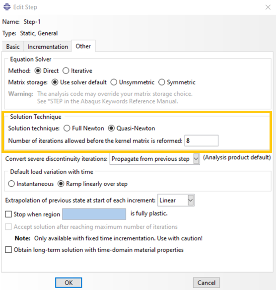
Figure 7: Selecting the ‘Quasi-Newton’ technique and number of iterations between stiffness matrix reformation
3. Summary
In this post we explained the distinction between linear and non-linear problems in finite element analysis (FEA). FEA simulations aim to mirror real-world scenarios.
Linear problems exhibit a direct proportionality between input and output. Imagine stretching a spring – the applied force increases steadily with the distance stretched. Non-linear problems deviate from this simplicity. Bending a metal wire is an example. It bends easily at first, but resistance increases significantly as you push further. Abaqus offers linear and non-linear analysis tools to handle these different responses.
Also, we dived into the key characteristics of both problem types, along with the various sources of non-linearity that FEA engineers frequently encounter. These sources are:
- Geometric non-linearity: This occurs when the magnitude of displacements affects the structure’s response. Large deflections or rotations, and “snap-through” behavior (where a structure suddenly switches from one stable position to another) are examples.
- Material non-linearity: This arises when the material’s response to applied loads deviates from the linear relationship between force-displacement or stress-strain. Rubber is a typical example – it exhibits a non-linear stress-strain curve.
- Boundary non-linearity: This occurs when the boundary conditions change during the analysis. Imagine a beam that starts tipping freely but then hits a stop, introducing a new constraint.
Understanding these non-linear sources is crucial for choosing the appropriate analysis approach and achieving accurate simulations in Abaqus (Abaqus nonlinear).
One last note:
As you know, nonlinear analyses most probably lead to convergence issues in Abaqus. So, how do you plan to overcome them? Do you even know what does convergence mean?
I suggest to read this article “Abaqus convergence” to get all of your answers.
Also, we have a special offer for you to learn this whole nonlinearity and convergence like a pro with practical examples (Abaqus nonlinear). You just need to watch this package: “Abaqus convergence tutorial | Introduction to Nonlinearity and Convergence in ABAQUS”
 |
This package introduces nonlinear problems and convergence issues in Abaqus. Solution convergence in Abaqus refers to the process of refining the numerical solution until it reaches a stable and accurate state. Convergence is of great importance especially when your problem is nonlinear; So, the analyst must know the different sources of nonlinearity and then can decide how to handle the nonlinearity to make solution convergence. Sometimes the linear approximation can be useful, otherwise implementing the different numerical techniques may lead to convergence. Through this tutorial, different nonlinearity sources are introduced and the difference between linear and nonlinear problems is discussed. With this knowledge, you can decide whether you can use linear approximation for your nonlinear problem or not. Moreover, you will understand the different numerical techniques which are used to solve nonlinear problems such as Newton-Raphson. All of the theories in this package are implemented in two practical workshops. These workshops include modeling nonlinear behavior in Abaqus and its convergence study and checking different numerical techniques convergence behavior using both as-built material in Abaqus/CAE and UMAT subroutine. |
It would be helpful to see Abaqus Documentation to understand how it would be hard to start an Abaqus simulation without any Abaqus tutorial.
One note, when you are simulating in Abaqus, be careful with the units of values you insert in Abaqus. Yes! Abaqus don’t have units but the values you enter must have consistent units. You can learn more about the system of units in Abaqus.
Also, click on this link to learn about: “Automatic Stabilization Abaqus of Unstable Problems“.
Moreover, the general description of how to write a subroutine is available in the article titled “Start Writing a Subroutine in Abaqus: Basics and Recommendations “. If you even do not familiar with the FORTRAN, you can learn the basics via this article: “Abaqus Fortran “Must-Knows” for Writing Subroutines”. You may also like this article to begin writing your own UMAT: “Start Writing Your First UMAT in Abaqus”