
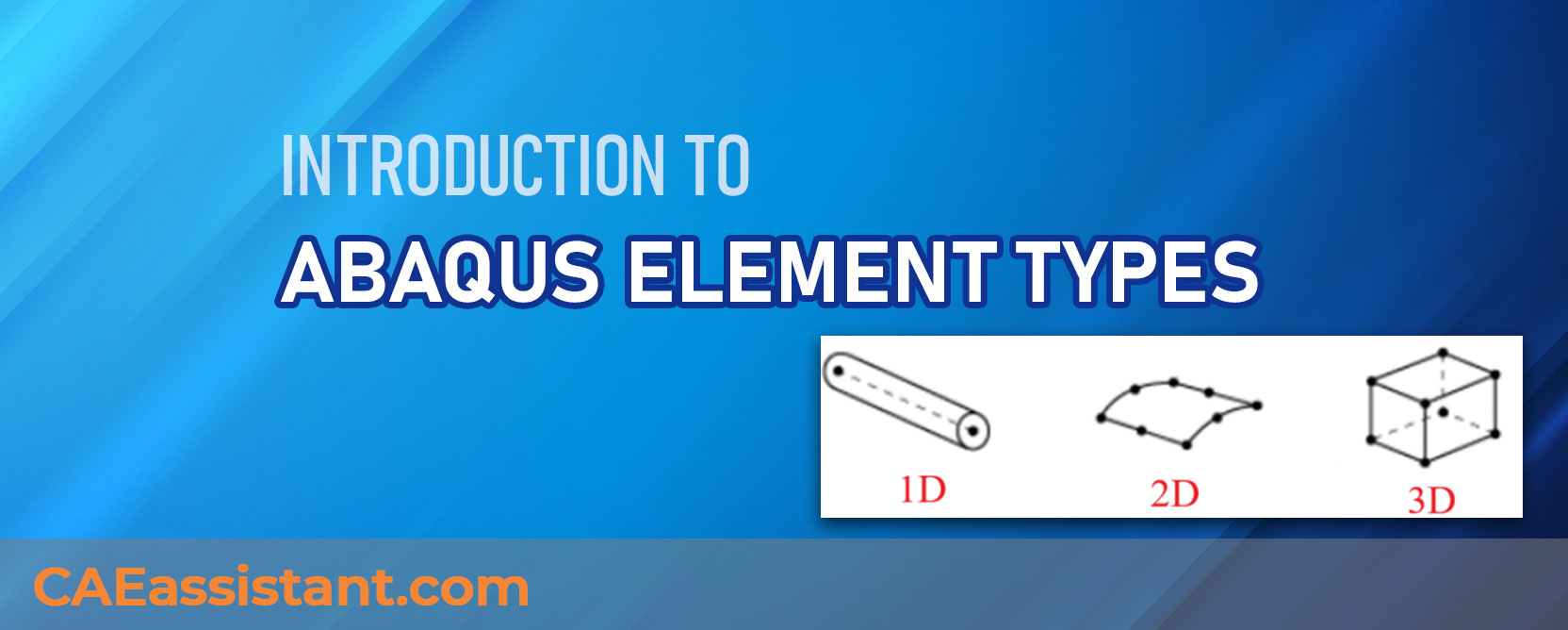
Introduction to Abaqus element types
Stuck on choosing Abaqus element types for your simulation? Now, let me ask you a question, Do you even familiar with them? As you know, Choosing the right element type is important, and Abaqus element library offers a variety of options!
This post will give you a breakdown of Abaqus element types, categorized in a few key ways. To give you a tip before we start, there are five aspects (maybe more) you can categorize the element types. So, let’s dive in.
1. Introduction to Abaqus element types
Knowing the Abaqus element types is the first step to understand the Abaqus elements and finally selecting the proper element type for your simulation. The Abaqus elements can be categorized in 5 aspects:
- Family
- Number of Nodes
- Degrees of Freedom
- Formulation
- Integration
Let’s define each of them.
1.1. Family
A family of finite elements is the most general way to group different types of elements. It’s like a big umbrella category that covers all the specific types of elements that can be used. The major distinction between the element families is the geometry that each family assumes.
You can see the common element families in figure 1.
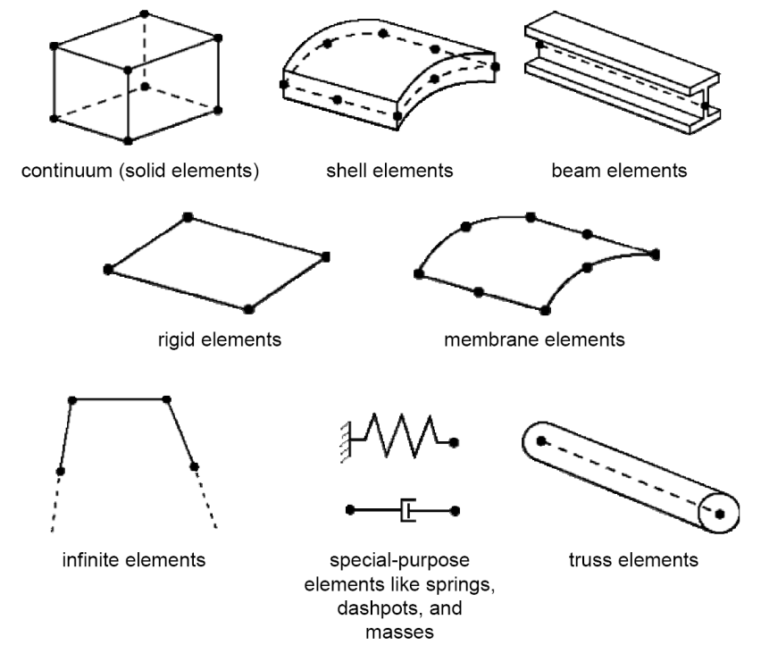
Figure 1: Common element families
1.2. Number of nodes (Interpolation)
Imagine building blocks that come together to form complex structures. These building blocks, in the world of finite element analysis (FEA), are called elements. Each element is made up of connection points called nodes. The number of nodes in an element act like a control knob. More nodes allow for greater freedom of movement (degrees of freedom) for the element, making it more flexible and able to bend and deform more realistically.
This ability to deform is further influenced by how we interpolate, or estimate, the behavior between these connection points. The number of nodes dictates the strategy used for this interpolation. There are two main approaches within Abaqus (and most other advanced solvers): linear and quadratic.
- First-Order (Linear): This approach works best for elements with nodes only at their corners, like triangles with three nodes. However, it can only represent a constant state of strain within the element, limiting its ability to capture complex deformations.
- Second-Order (Quadratic): This approach is more versatile and is used for elements with both corner nodes and mid-side nodes, like quadrilaterals with four nodes. Quadratic interpolation allows for a more gradual change in behavior within the element, leading to more realistic simulations of bending and deformation.
See figure 2 to better understand the first-order and second-order interpolation.
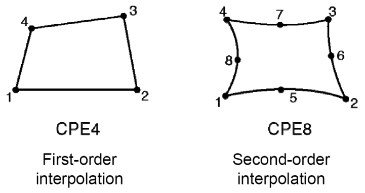
Figure 2: First-order & Second-order interpolation
1.3. Degrees of freedom
In an element, each node has various degrees of freedom (DOF) – essentially unknowns the analysis solves for. These DOF dictate how the element will behave under stress.
These DOF reside at the element’s nodes and represent fundamental physical quantities, such as:
- Displacements: How much a node can move in different directions (e.g., up/down, left/right).
- Rotations: How much the element can twist or turn.
- Temperature: The temperature variation within the element (for thermal analysis).
- Electrical Potential: The voltage at the node (for electrical analysis).
1.4. Formulation
Another way to categorize elements in finite element analysis (FEA) is by the math equations used to describe their behavior. These equations essentially act as a blueprint that dictates how the element will respond to forces and deformations.
To model the behavior of small parts (elements) within a larger system. There are two main formulations:
- Lagrangian: The elements move and deform along with the material they represent. This is good for analyzing things like stress and displacement in solids.
- Eulerian: The elements stay fixed in space, and the material flows through them. This is better for simulating fluids.
Within these two main types, there can be additional variations to account for specific situations. For example, with shells (curved elements), there are options for thin or thick shells depending on the stress conditions.
Some other additional variations:
- Plane strain
- Small-strain shells
- Plane stress
- Finite-strain shells
- Hybrid elements
- Incompatible-mode elements
1.5. Integration
Now, the question is how and where to implement these formulations in the finite element analysis. This is where the Integration comes into play.
Abaqus uses a numerical method called integration to calculate material behavior within an element. Imagine dividing the element up into a bunch of small points (integration points). The software then figures out how the material behaves at each of these points. More integration points provide more accurate results, but take more computer power to solve.
To improve efficiency, Abaqus offers a “reduced integration” option that uses fewer integration points. This can significantly speed up calculations. However, be careful! Using reduced integration incorrectly can lead to inaccurate or misleading results in your analysis.
See figure 3 to understand the integration options and to see its relation with the interpolation.
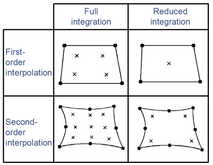
Figure 3: Full integration & Reduced integration
2. Introduction to Abaqus element dimension
Now comes the question: how do we choose the right element for our model? Since multiple types of elements might be applicable for a single model, which one should we use? The common answer from most analysts is to choose the element that simplifies the simulation to implement the problem’s physics.
To address this, we first need to determine the problem’s dimensionality (1D, 2D, or 3D). Abaqus element library covers this situation with the following categories:
- 1D elements
- 2D elements
- 3D elements
- Cylindrical elements
- Axisymmetric elements
This classification represents another way (aspect) of categorizing elements. But before we define each category above, let’s see the difference between the spatial dimensions of the problem and the dimensions of the elements.
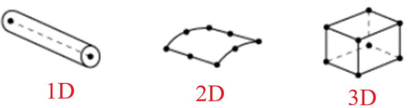
Figure 4: Element dimensions
2.1. Spatial dimensionality VS Element dimensionality
Imagine you’re building a model of a car using Legos for a special project. Here’s how spatial dimensionality and element dimensionality come into play:
- Spatial Dimensionality: This refers to the actual number of dimensions the entire car exists in, which in our case is 3D (three-dimensional). The car has length, width, and height.
- Element Dimensionality: This refers to the number of dimensions needed to define a single Lego brick. Most Lego bricks we use are simple and can be defined by their 1D (one-dimensional) length. You only need one number (the length) to know the size of the brick.
However, things get interesting when we consider more complex Lego pieces:
- Example 1: Beam Lego Brick: This brick might be long and thin, similar to a real beam. Even though the brick itself can be defined by its length (1D), the beam Lego piece is designed to represent a real-world beam that has width and thickness (in 3D space). So, the element dimensionality is 1D, but it contributes to a 3D spatial model.
- Example 2: Lego Plate: This flat plate can be defined by its length and width (2D). Similar to the beam, the Lego plate represents a real-world object with a certain thickness (3D). So, the element dimensionality is 2D, but it contributes to a 3D spatial model.
The Key Takeaway:
- Spatial dimensionality tells you how many dimensions the entire model/object occupies (e.g., the car is 3D).
- Element dimensionality tells you how many dimensions are needed to define a single building block of the model (e.g., most Lego bricks are 1D, while plates are 2D).
- Even though element dimensionality might be lower, it can still represent objects in a higher dimensional space (e.g., Lego bricks and plates contribute to a 3D car model).
2.2. 1D elements
- Sometimes referred to as “Link” or “Line” elements.
- Can be used to transmit loads and fluxes
- Commonly used for long membered structures
- Define by two nodes
- It is not suitable for modeling complex geometries or localized stresses (e.g. stress concentration, notch, hole)
Imagine you are building a simple model with beams. These beams are like one-dimensional elements. They are easy to use for long, thin structures and can represent how stiff the whole structure is. They are also good at showing the overall stress in the structure. However, they cannot handle very complex shapes or show you exactly where the stress is highest (like at a sharp corner).
2.3. 2D elements
- They are represented geometrically in 2 dimensions.
- Can be triangular (3 nodes, 3 mid-side nodes in case of second-order) or quadrilateral (4 nodes, 4 mid-side nodes in case of second order)
- Planar: for example shell element
- Common ones are plane stress and plane strain
Two-dimensional elements (2D) are like flat shapes, either triangles or squares, used to build models in two dimensions. They can be used for flat objects or even to represent slices of 3D objects. These elements are great for analyzing things like stress in a flat sheet of metal or the forces in a thin wall.
2.4. 3D elements
- Often referred to as solid elements
- Spatial dimensionality and element dimensionality are one.
- Used when geometry or loading conditions are too complex.
- What you see is what you get (mostly).
Imagine building a model with actual 3D objects, like cubes or other shapes. These are 3D elements. They are best when the shape you’re modeling is complex or the forces acting on it are coming from all directions. Since the model is fully 3D, the results you get (like stress or strain) will also be 3D, showing exactly how everything is affected in all directions.
2.5. Cylindrical elements
- Special class of solid elements
- Used to model structures with circular or axisymmetric geometry subjected to non-axisymmetric loading.
- For curve shape of circular objects, less mesh refinement and so less computational power needed.
2.6. Axisymmetric elements
- Axisymmetric elements are for rotationally symmetric bodies about a central axis.
- They require axisymmetric loading conditions (except for advanced formulations).
- Axisymmetric loading and geometry allow 2D elements to model 3D bodies.
- Stresses are independent of rotational angle in axisymmetric problems.
- A single 2D plane (element) represents a 3D space for axisymmetric problems.
- Example: thick-walled, cylindrical pressure vessel under internal pressure.
3. Summary
In this blog post, we tried to introduce Abaqus element types, which are essential for finite element analysis (FEA) simulations. The right element type selection can significantly impact the accuracy and efficiency of your simulation.
The blog categorizes Abaqus elements into five key aspects: family, number of nodes, degrees of freedom, formulation, and integration. It explains each aspect in detail with figures to illustrate the concepts. For instance, under the family aspect, it covers common element families like solid, shell, beam, etc.
Then, we dived into element dimensionality (1D, 2D, 3D, etc.) and clarified the difference between spatial dimensionality and element dimensionality. It highlights that even lower-dimensional elements can represent higher-dimensional objects. Finally, it explains different types of elements based on dimensionality, including 1D elements (beams), 2D elements (plates), 3D elements (solids), cylindrical elements, and axisymmetric elements.
Now, you have learned the basic stuff about the Abaqus element types, but what is the difference between element and mesh? read this article to understand that: “Mastering the Abaqus Mesh: A Guide to Meshing Techniques in Abaqus“
Also, you can always learn more from the Abaqus documentation.
Or you can find valuable info about specific types of elements such as Membrane and shell in this article: Shell VS Membrane
But some questions still remained like:
- How to select the best element type for my simulation?
- How to name the elements?
- What are continuum elements?
- …
Stay tuned with us and we will answer all these questions in the next blogs. Abaqus element types
Wish you the best.
Explore our comprehensive Abaqus tutorial page, featuring free PDF guides and detailed videos for all skill levels. Discover both free and premium packages, along with essential information to master Abaqus efficiently. Start your journey with our Abaqus tutorial now!