1. Introduction| Abaqus Thermal Expansion Behavior Simulation
In this tutorial, the user subroutines UEXPAN and VUEXPAN are used to simulate the thermal expansion behavior of a linear elastic material. The geometric model used in this study is a two-dimensional square specimen under temperature loading.
This subroutines are used when the material’s thermal expansion behavior is too complex to model with the “EXPANSION” option in the Abaqus software environment. For example, the subroutines are used in problems where the thermal strains are complexly dependent on temperature, predefined field variables, and state variables, and there is a need to update these variables.
This project is designed to enhance participants’ understanding how to accurately simulate the complicated thermal expansion models of the materials using UEXPAN and VUEXPAN subroutines.
2. Simulation of the Thermal Expansion Behavior of a Linear Elastic Material using UEXPAN and VUEXPAN Subroutine (PDF File)
This project, after teaching the basic fundamentals of thermal expansion, presents seven examples of isotropic and orthotropic thermal expansion behaviors to teach the UEXPAN or VUEXPAN subroutine. The implementation of thermal expansion in these examples are done with UEXPAN subroutine for Abaqus/Standard solver (implicit method) and VUEXPAN for Abaqus/Explicit solver.
2.1. Problem Description
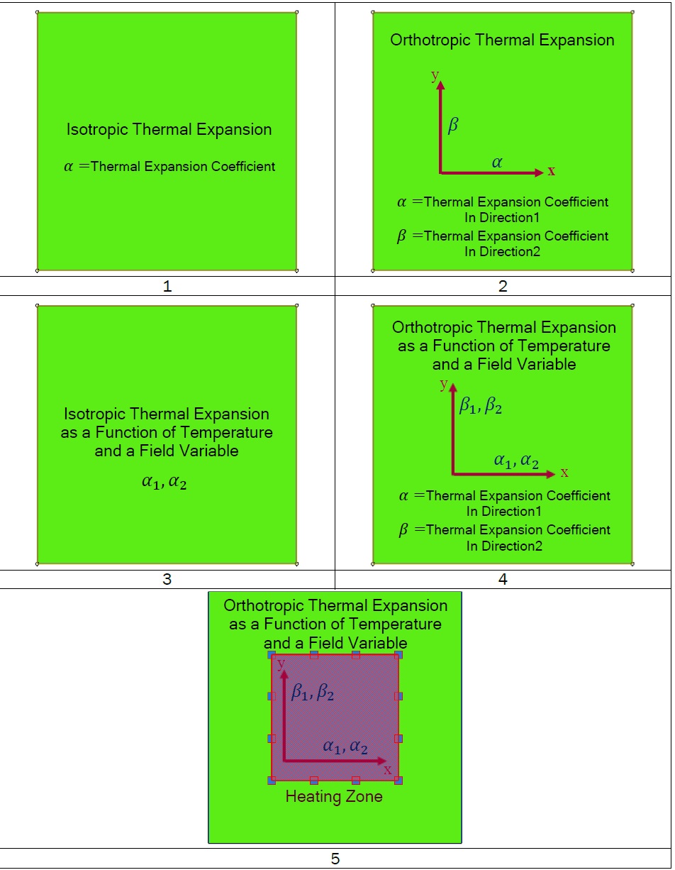
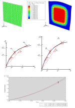
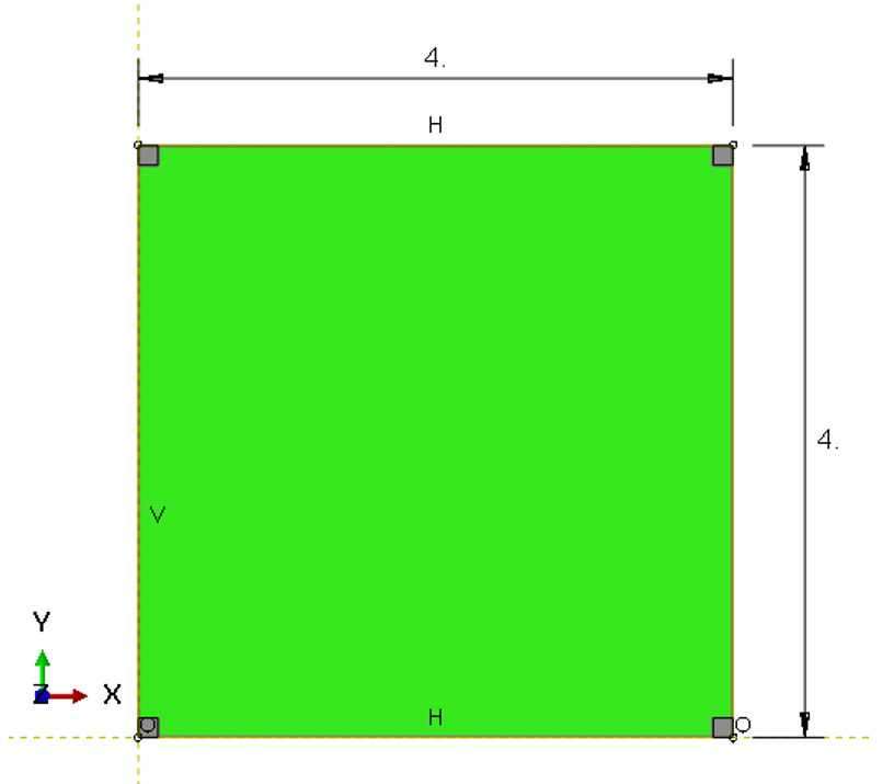
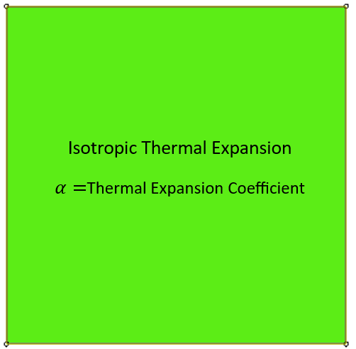
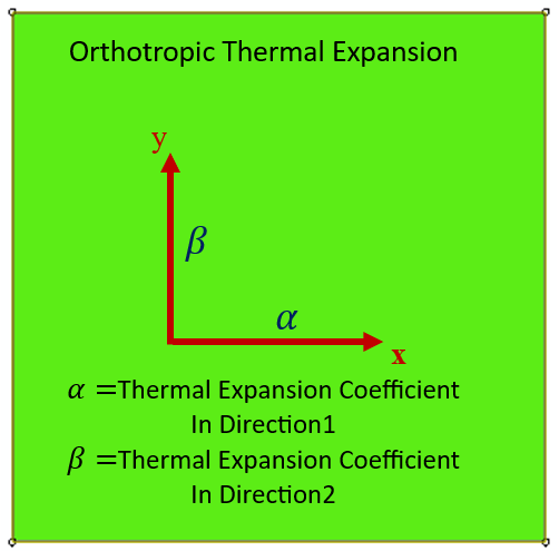
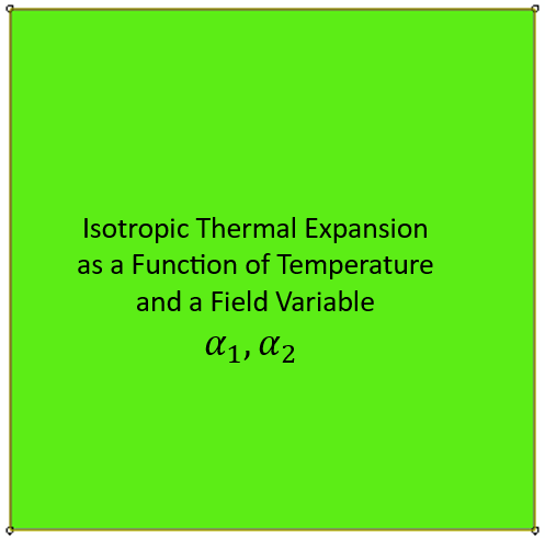
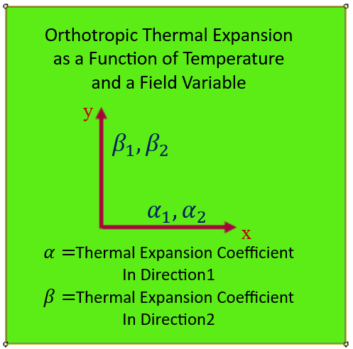
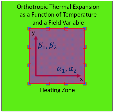
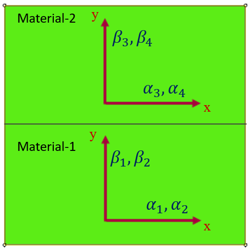
Geometry: The geometric model used in this study is a two-dimensional square specimen under temperature loading. The schematic design of the part is shown in Figure 1. This tutorial contains six examples to teach the UEXPAN subroutine, and one example for VUEXPAN subroutine. These examples are shown in Figure 2.
The material properties used in these examples are young’s modulus (E=1e6 Pa) and Poisson’s ratio (ϑ=0.3) for material-1, and young’s modulus (E=0.6e6 Pa) and Poisson’s ratio (ϑ=0.27) for material-2.
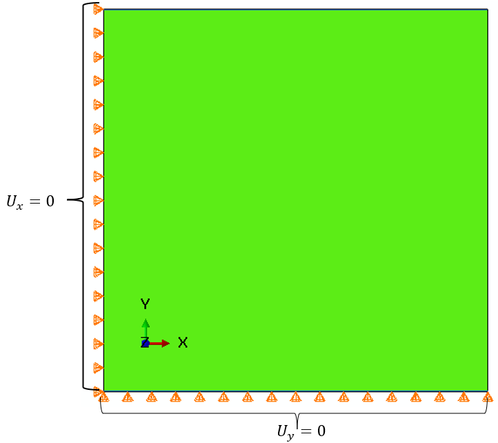
The temperature of the specimen is set to 100 degrees Celsius. The boundary conditions of model are shown in Figure 3.
Figure 1: The schematic design of the two-dimensional square specimen
1 |
2 |
3 |
4 |
5 |
6 |
Figure 2: The six examples of the tutorial
Figure 3: The displacement boundary conditions
2.2. Project Procedures
- Setting up the software environment and choosing Abaqus units;
- Creating the two-dimensional square specimen;
- Defining the material properties and creating its relevant section;
- Making an independent instance of the model in the “Assembly” module;
- Creating a “Static, Linear perturbation” step and a “Static, General” step for doing analysis by calling the UEXPAN subroutine or “Explicit” step for VUEXPAN;
- Determining the initial and boundary conditions, etc.;
- Generating elements and assigning element types;
- Preparing the UEXPAN or VUEXPAN subroutines for all the examples of the tutorial;
- Creating seven jobs and calling the relevant UEXPAN or VUEXPAN subroutines;
- Submitting the jobs;
- Viewing the results.
2.3. Executing Project Procedures
- Setting up the software environment
Geometry:
The geometric model used in this study is a two-dimensional square specimen under temperature loading. The schematic design of the part is shown in Figure 1.
Material Properties:
The material properties used in these examples are young’s modulus (E=1e6 Pa) and Poisson’s ratio (ϑ=0.3) for material-1, and young’s modulus (E=0.6e6 Pa) and Poisson’s ratio (ϑ=0.27) for material-2.
Steps:
The thermal expansion analysis procedure for these examples would be a “Static, Linear perturbation” step and a “Static, General” step for doing analysis by calling the UEXPAN subroutine. For the VUEXPAN subroutine, an “Explicit” step is called.
Boundary Conditions:
The left and lower edges of the part are restrained by using the displacement boundary conditions, as illustrated in Figure 2 (Ux = 0 for left edge and Uy = 0 for lower edge).
Meshing:
For Abaqus/Standard solver, the meshing operation was performed using 4-node bilinear plane strain quadrilateral elements (CPE4).
- Preparing the subroutine
The basic fundamentals of thermal expansion, the description of UEXPAN and VUEXPAN subroutines variables, and all the UEXPAN and VUEXPAN subroutines used in this tutorial are explained in detail in section “Theoretical and Base Relations”.
- Creating the jobs and calling the relevant UEXPAN or VUEXPAN subroutines
- Submitting the jobs
- Guidance on how to extract the results
In the video file, the process of extracting the results is shown in full details.
2.4. Theoretical and Base Relations
Before introducing and describing the UEXPAN or VUEXPAN subroutine variables, it is necessary to briefly teach the basic fundamentals of thermal expansion.
1-Thermal Expansion
Thermal expansion is the mechanical tendency of a material to an increase in size (length, area, or volume), and changing its density, with increasing temperature. As we know, temperature is a function of the average molecular kinetic energy of a material. When a material is heated, the molecules begin to vibrate faster and move more. As the energy in the particles increases, they move faster and the intermolecular forces between them weaken, thus expanding the matter.
- Isotropic Thermal Expansion
- Orthotropic Thermal Expansion
- Anisotropic Thermal Expansion
- Calculation of Thermal Strains in the “Linear Perturbation” Steps
- Calculation of the Thermal Stresses
2-The UEXPAN Subroutine
2-1- The General Form of UMAT Subroutine
2-2- Introduction of Variables
2-3- Variables to be Defined by the User
- EXPAN (*)
- DEXPANDT (*)
3- The UEXPAN Subroutines used in This Tutorial
3- 1- The UEXPAN Subroutine for Isotropic Thermal Expansion Behavior (1_UEXPAN_ISOTROPIC)
3- 2- The UEXPAN Subroutine for Orthotropic Thermal Expansion Behavior (2_UEXPAN_ Orthotropic)
3- 3- The UEXPAN Subroutine for Isotropic Thermal Expansion Behavior Considering a Field Variable
(3_ UEXPAN_ISOTROPIC_FV)
3- 4- The UEXPAN Subroutine for Orthotropic Thermal Expansion Behavior Considering a Field Variable
(4_ UEXPAN_ Orthotropic _FV)
3- 6-The UEXPAN Subroutine for Orthotropic Thermal Expansion Behavior Considering a Field Variable
for Two materials using NOEL Variable (6_ UEXPAN_ Orthotropic _FV_NOEL):
4- The VUEXPAN Subroutine
3. Workshop (Video File): A step-by-step guide on the simulation of thermal expansion behaviors using UEXPAN and VUEXPAN subroutines
The workshop provides a full step-by-step guide through a video to simplify the simulation of the complicated thermal expansion models using UEXPAN and VUEXPAN subroutines. In the video, how to model, call subroutines, submit the jobs and extract results is shown in full detail.
Results
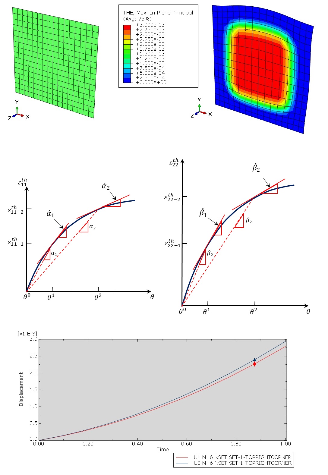
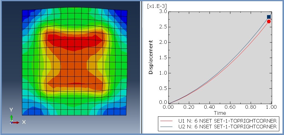
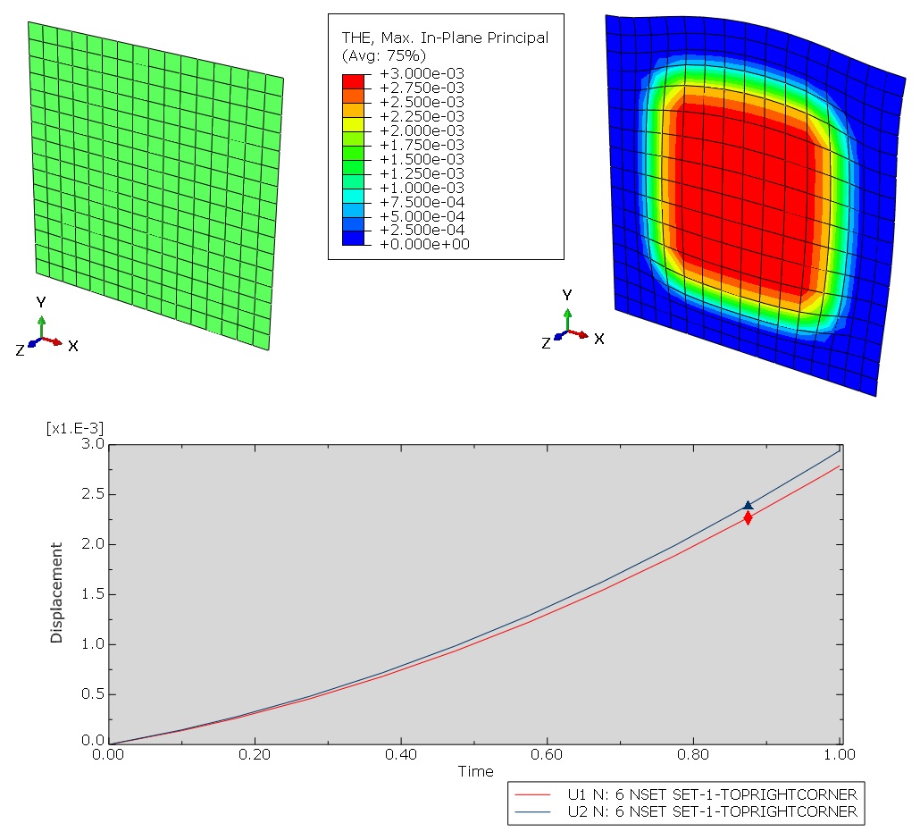
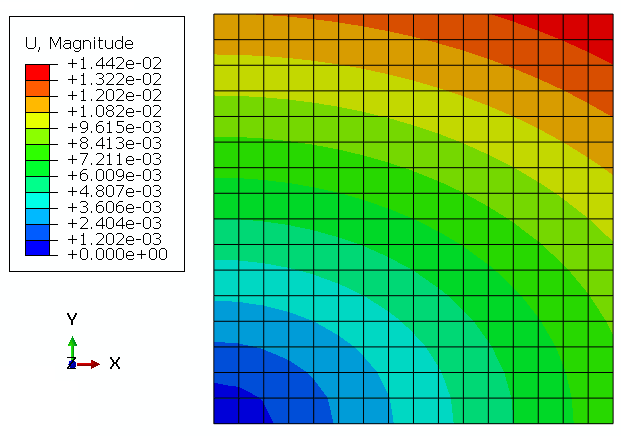
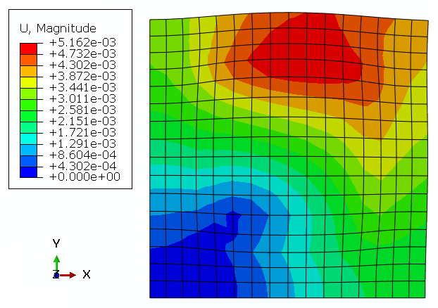
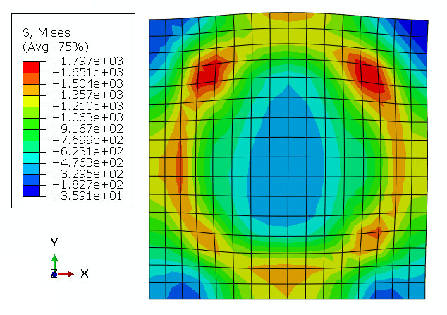
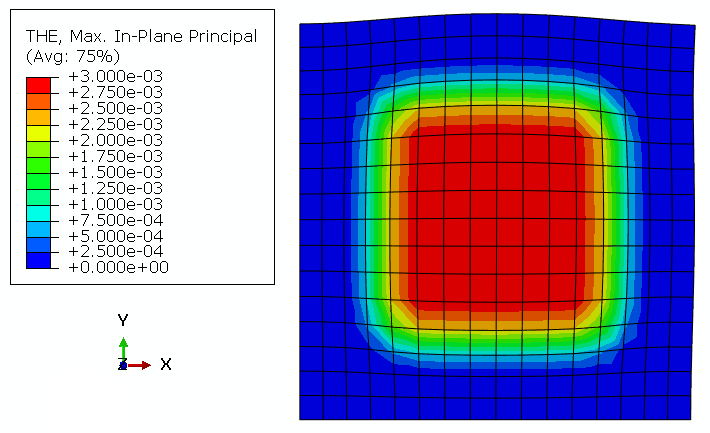
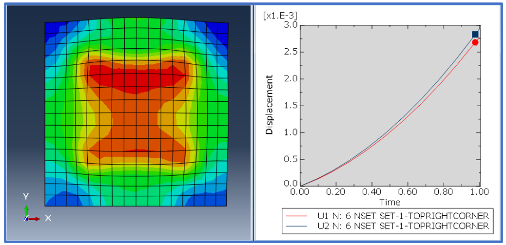
The stress distribution field (S), displacement distribution field (U), strain distribution field (), thermal strain distribution field (), reaction forces (RF), displacement-time diagram (U-t), etc., are the output results of this analysis.
Figure 4: Displacement-time diagram
It would be helpful to see Abaqus Documentation to understand how it would be hard to start an Abaqus simulation without any Abaqus tutorial.
One note, when you are simulating in Abaqus, be careful with the units of values you insert in Abaqus. Yes! Abaqus don’t have units but the values you enter must have consistent units. You can learn more about the system of units in Abaqus.
Reviews
There are no reviews yet