
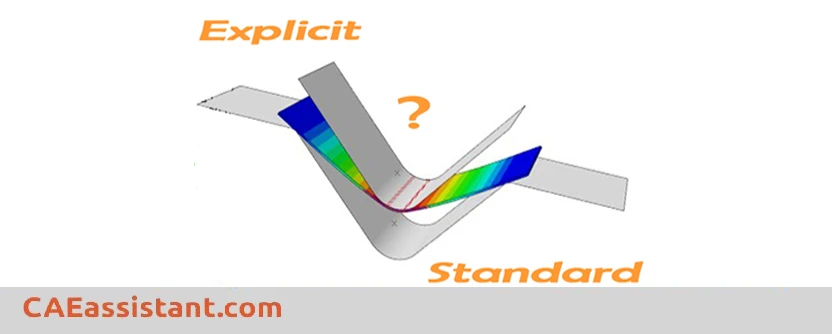
1. Abaqus Explicit or Abaqus Implicit?
Have you ever wondered, “Abaqus Standard or Abaqus Explicit?” It’s a common question when you’re gearing up for your analysis. Aside from the specialized CFD solver (Abaqus/CFD) designed for fluid problems, Abaqus revolves around its two core analysis modules: Abaqus Implicit and Abaqus Explicit. In this post, we’re about to unveil the key differences between these two solvers and help you pick the one that’s just right for your analysis needs. Stick around with CAE Assistant!
2. Abaqus implicit and Explicit Solvers | Abaqus standard vs implicit!
First, I have to say that there are no differences between Abaqus Standard and Implicit. In fact, these are two names for one solver. The main discussion is about Abaqus Implicit and Abaqus Explicit solvers.
These solvers are based on two approaches in FEM analysis, namely implicit (for Abaqus/Standard) and explicit. The distinction between the two different numerical approaches makes it possible to understand which solver to use.
Read More: Debugging of ABAQUS errors
In the case of the implicit method, equilibrium is enforced between externally applied load and internally generated reaction forces at every solution step (Newton Raphson method).
In the case of the Abaqus explicit method, there is no enforcement of equilibrium. But this does not mean that explicit is not accurate. You can minimize its deviation from equilibrium to almost zero by increasing the number of solution steps, i.e. reducing the time step size.
We can list the main differences below:
Abaqus Implicit is unconditionally stable.
Implicit schema is incremental as well as iterative. However, explicit schema is only incremental.
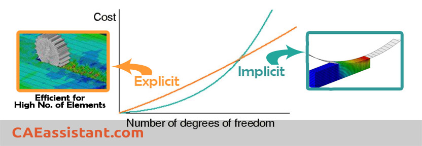
In terms of cost per Increment, it is costly for implicit and cheaper for explicit. Disk space and memory usage are typically much smaller than that for implicit. The explicit method shows great cost savings over the implicit method as the model size increases:
Therefore, Abaqus/Standard(or Abaqus implicit) must iterate to determine the solution to a nonlinear problem but Abaqus/Explicit determines the solution without iterating by explicitly advancing the kinematic state from the previous increment. Read More: Quasi Static

3. Explicit or Standard, Which one should I use?
For many analyses, it is clear whether Abaqus/Standard or Abaqus/Explicit should be used. For example, Abaqus/Standard is more efficient for solving smooth nonlinear problems; on the other hand, Abaqus/Explicit is the clear choice for high-speed dynamic analyses such as crash analysis or drop test. There are, however, certain problems that can be simulated well with either program.
Typically, these are problems that usually Abaqus/Standard can solve but may have difficulty converging because of contact or material complexities, resulting in a large number of iterations. For example, in problems where very complex contact conditions or very large deformations are present. Such analyses are expensive in Abaqus/Standard because each iteration requires solving a large set of linear equations.
4. The Maximum Increment Size in Abaqus: Implicit vs Explicit Solvers
Have you ever explored the concept of the maximum increment size in Abaqus for Implicit vs Explicit solvers? Are you aware that there are separate criteria for controlling the increment size in Abaqus Standard and Abaqus Explicit? These are fundamental concepts that Abaqus users must understand, and we have explored them here.
4.1. The Maximum Increment Size in Abaqus Explicit
Abaqus Explicit does not check the convergence of the solution. Therefore, using large time increments in Abaqus Explicit can lead to unreal oscillations or sudden material failure. The below figure shows how a large time increment modifies the results in Abaqus Explicit simulations. So, we must ensure that the stability condition is checked during the solution process. To do so, we need to calculate the stable increment size. Two options are available for defining the stable increment size in Abaqus Explicit: Automatic and Fixed. We will discuss them in detail in the following.
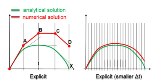
Figure – The effect of increment size on the results for Explicit solvers [1].
4.1.1 Automatic Time Incrementation
Abaqus Explicit uses an approximated method to ensure that the solution remains stable. This is achieved by setting the maximum increment size to be less than the stable time increment. There are two options for automatically calculating the stable time increment in Abaqus Explicit: “global” estimation and “element-by-element” estimation.
The element-by-element method limits the maximum increment size to the constant value in Equation (1).
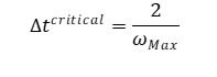 |
(1) |
Where ωmax is the largest frequency in the model. Abaqus Explicit calculates the frequency for each element based on the material properties and the element size. The below figure provides instructions on how to select the “Element-by-element method” in the “Edit Step” window in Abaqus.
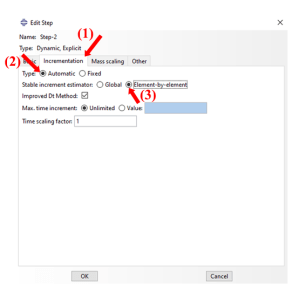
Figure – Choosing the Element-by-element method in the Abaqus “Edit Step” window.
The element-by-element method does not consider the effects of boundary conditions and contacts, during the solution, on the maximum increment size. This may lead to unnecessarily large increment sizes and inefficient analysis.
To overcome the limitation of the element-by-element method in updating the model’s frequency, Abaqus Explicit offers the global estimation option. Global estimation updates the maximum increment size based on the real-time state of the model. This allows for larger time increments compared to the element-by-element method, making it more computationally efficient. Abaqus Explicit employs the global estimation method by default.
4.1.2 Fixed Time Incrementation
In some scenarios, the analysis requires an accurate representation of higher-mode responses. For such cases, the user must specify a smaller increment size relative to the element-by-element or global methods. This is where the fixed method becomes valuable. The below figure shows how to define a fixed increment size in an Abaqus Explicit step.
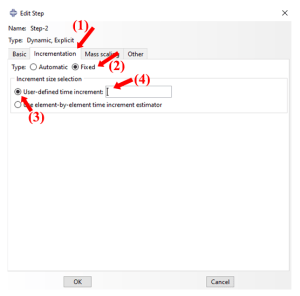
Figure – Choosing the Fixed method in the Abaqus “Edit step” window.
It is important to note that when using a fixed increment size, Abaqus does not check the stability condition. So, it is crucial to carefully select a fixed increment size that guarantees stable results.
4.2 The Maximum Increment Size in Abaqus Standard
In the Abaqus Standard, unlike the Abaqus Explicit, convergence must be checked at each increment. Therefore, we are less likely to experience instability issues related to the increment size. You can employ significantly larger increment sizes, without limitations, in Abaqus Implicit vs Explicit solvers. Moreover, the Abaqus Standard can automatically reduce the defined increment size to prevent converge issues. However, you must be careful not to choose an increment size that is too large. In this situation, Abaqus breaks the increments repeatedly due to convergence issues. This negatively affects the computational cost.
According to the below figure, the Abaqus Standard’s increment size has no significant impact on the analysis results. So, the Abaqus Standard is a more reliable choice compared to the Abaqus Explicit. However, achieving convergence within an increment may require numerous iterations or may not always occur. This highlights a significant limitation of Abaqus Implicit vs Explicit solvers.
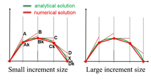
Figure – The effect of increment size on the results for Abaqus Standard solver [1].
4.3 Implicit vs Explicit Solvers: Which One to Choose
You are now familiar with the concept of maximum increment size in Abaqus implicit vs Explicit solvers. In the Abaqus Explicit, we typically use a greater number of steps compared to the Abaqus Standard. However, the computational effort required to solve each increment is generally high in the Abaqus Standard. You may wonder how to decide between the Abaqus solvers for a specific problem. There is no absolute instruction. Choosing the right solver requires experience and depends on the specific characteristics of your problem.
In the video below, prepared by the CAE Assistant team, see the complete comparison between the Abaqus standard solver and the Abaqus explicit solver:
Until now, we have tried to explain ‘Abaqus standard and Abaqus explicit’ thoroughly so that you can choose the right solver for your needs. Also we clarified there is no difference between Abaqus standard vs implict. they typically refer to the same solver.
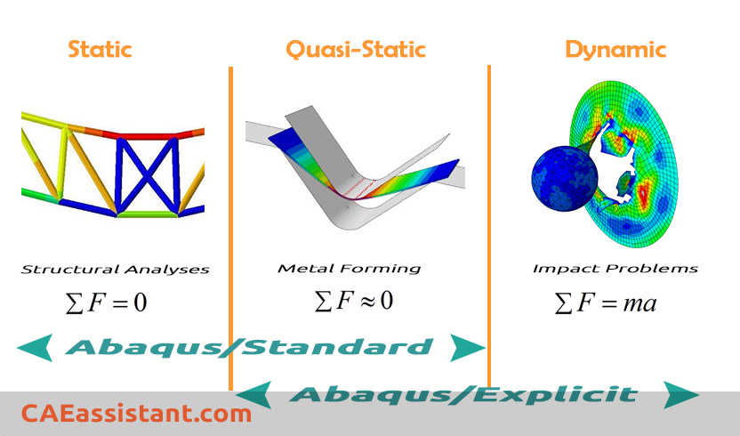
5. Indicating Quasi-static Analysis
How can I know my simulation is quasi-static or not?
5.1 What is quasi-static analysis?
In summary, in quasi-static analysis, the assumption is made that the problem can be treated as static at any specific moment in time. The key concept is that the applied loading changes very gradually, with a frequency significantly lower than that of the structure. As a result, the structure deforms as if it were under static conditions, and the influence of inertia is considered negligible. This assumption is effective when the effects of inertia are minimal, and it allows for the simplification of non-linear problems into linear systems.
In long term, Quasi-static analysis is a method used in engineering and physics to analyze the behavior of a system or structure under slowly varying loads or conditions. It is a simplified approach that assumes the system remains in equilibrium at each stage of the analysis, neglecting the dynamic effects and considering only the static forces.
In quasi-static analysis, the system is divided into a series of static equilibrium states, and the response of the system is determined at each step. The applied loads are assumed to change gradually or incrementally, allowing the system to adjust and reach a new equilibrium at each stage. This analysis technique is often used when the dynamic effects, such as inertia, vibration, and time-dependent behavior, can be considered negligible compared to the static forces and deformations.
Quasi-static analysis is commonly employed in various fields, including structural engineering, mechanical engineering, civil engineering, and materials science. It helps engineers and researchers understand how a structure or system will respond under various loads and allows for the calculation of stresses, strains, displacements, and other relevant parameters. By simplifying the analysis to static equilibrium states, it provides a practical and efficient approach for predicting the behavior of systems subject to slow or gradual changes.
5.2 Difference between quasi-static analysis and dynamic analysis
The main difference between quasi-static and dynamic analyses lies in the consideration of time-dependent effects and the assumption of equilibrium.
Quasi-static analysis assumes that the system or structure remains in equilibrium at each stage of analysis and neglects the dynamic effects such as inertia, vibration, and time-dependent behavior. It is suitable for situations where the time scale of the loading or the response is much larger than the characteristic time scale of the dynamic effects. Quasi-static analysis is computationally simpler and often provides a reasonable approximation for slowly varying or static loads.
On the other hand, dynamic analysis explicitly accounts for the time-dependent behavior of a system or structure. It considers the effects of inertia, damping, and time-varying forces. Dynamic analysis is necessary when the time scale of the loading or the response is comparable to or larger than the characteristic time scale of the dynamic effects. It is used to study the behavior of structures subjected to rapid or impulsive loads, seismic events, vibrations, and other dynamic phenomena.
While quasi-static analysis is simpler and computationally less demanding, dynamic analysis provides a more accurate representation of the system’s behavior under time-varying conditions. However, there are cases where a combination of both approaches is needed.
In dynamic analysis, there are situations where quasi-static analysis is used as part of the overall analysis. This can occur when the dynamic response is dominated by certain frequencies or modes of vibration. In such cases, the dynamic analysis may be separated into two parts: a quasi-static analysis to determine the response at low frequencies or during initial stages, and a dynamic analysis to capture the higher-frequency or time-dependent behavior. For example, in seismic analysis of structures, a quasi-static analysis may be performed to evaluate the response under the predominant low-frequency ground motions, followed by a dynamic analysis considering the higher-frequency components and the interaction between the structure and the ground.
5.3 Quasi-static analysis in Abaqus
As a rule of thumb, a simulation is static or quasi-static if the excitation frequency is less than 1/10 of the lowest natural frequency of the structure. This is mentioned in Abaqus Documentation:
“It is usually desirable to increase the loading time to 10 times the period of the lowest mode to be certain that the solution is truly quasi-static.“
In a static or quasi-static analysis, the lowest mode of the structure usually dominates the response. Therefore, knowing the frequency and, correspondingly, the period of the lowest mode, you can estimate the time required to obtain the proper static response. The natural frequencies can be calculated easily using the eigen frequency extraction procedure in Abaqus/Standard (Frequency analysis).
additionally, It would be useful to see Abaqus Documentation to understand how it would be hard to start an Abaqus simulation without any Abaqus tutorial. Also, please share your views with the CAE Assistant experts in the comment section. We really appreciate your feedback, as it helps us improve our tutorials and fulfill all your CAE needs without requiring additional tutorials.
 |
⭐⭐⭐ Abaqus Course | ⏰10 hours Video 👩🎓+1000 Students ♾️ Lifetime Access
✅ Module by Module Training ✅ Standard/Explicit Analyses Tutorial ✅ Subroutines (UMAT) Training … ✅ Python Scripting Lesson & Examples |
You can have the PDF of this post by clicking on CAE Assistant- Abaqus implicit or Abaqus explicit
Which of the Explicit or Standard solvers is more suitable for my problem?
Abaqus/Standard is a good choice to solve static, low-speed dynamic, steady-state transport, or smooth nonlinear analyses. On the other hand, Abaqus/Explicit is the clear choice for quasi-static events such as the rolling of hot metal, severely nonlinear behavior such as contact, transient response, or high-speed dynamic analyses such as crash analysis or drop test. There are, however, certain problems that can be simulated well with either program.
What are the main differences between Explicit and Implicit Solvers in Abaqus?
- Implicit is unconditionally stable.
- Implicit schema is incremental as well as iterative. However, the explicit schema is only incremental.
- In terms of cost per increment, it is costly for implicit and cheaper for explicit.
- Disk space and memory usage are typically much smaller than that implicit: look at this diagram.
What is the difference between the solving strategy of Abaqus/Standard and Abaqus/Explicit?
These solvers are based on two approaches in FEM analysis, namely implicit (for Abaqus/Standard) and explicit. The distinction between the two different numerical approaches makes it possible to understand which solver to use. Abaqus/Standard must iterate to determine the solution to a nonlinear problem, but Abaqus/Explicit determines the solution without iterating by explicitly advancing the kinematic state from the previous increment.
What methods are used to analyze problems in Implicit and Explicit Solver?
In the case of the implicit method, equilibrium is enforced between externally applied load and internally generated reaction forces at every solution step (Newton Raphson method).
In the case of the explicit method, there is no enforcement of equilibrium. But this does not mean that explicit is not accurate. You can minimize its deviation from equilibrium to almost zero by increasing the number of solution steps, i.e. reducing the time step size.
How can we solve problems that involve several analysis stages?
Abaqus provides a useful capability for simulations involving several analysis stages. In this ability, the user can start a simulation in Abaqus/Explicit. Then the results at any point within the solver run can be transferred as the starting point for continuation in Abaqus/Standard. The user will define new model information during the import analysis.
Thank you for being with us in this article. In order to always provide you with up-to-date and engaging content, we need to be familiar with your educational and professional experiences so that we can offer articles and lessons that are most useful to you.
Good write-up. I definitely appreciate this site. Keep it up! Elle Tanny Kirtley
Wow, superb blog layout! How long have you been blogging for? you make blogging look easy. The overall look of your website is excellent, as well as the content! Jacquelynn Kareem Ardyth