
Abaqus spring element(s) allow engineers to accurately represent physical springs and idealized axial or torsional components. By coupling forces with displacements or moments with rotations, these elements can exhibit both linear and nonlinear behaviors, making them highly versatile for various applications.
From modeling physical springs and structural dampers to restraining rigid body motion and performing frequency-dependent analyses, Abaqus Spring Elements prove indispensable. They are capable of temperature and field variable dependency, and they support both small and large displacement analyses. Whether you need a linear spring characterized by constant stiffness or a nonlinear spring with variable stiffness, Abaqus provides the tools to achieve realistic simulations.
In this article, we will delve into the features and applications of Abaqus Spring Elements. We will explore their different behaviors, types, degrees of freedom, and methods to model varying stiffnesses in compression and tension.
1. What is Abaqus Spring Element?
Abaqus Spring Elements are used to model the behavior of physical springs and idealized axial or torsional components within the Abaqus finite element analysis software. These elements can couple a force with a relative displacement or a moment with a relative rotation, and they can exhibit linear or nonlinear behavior. Spring elements can be dependent on temperature, field variables, and frequency, making them versatile for various engineering applications. In addition, they can be utilized to assign a structural damping factor, forming the imaginary part of spring stiffness.
Key features of Abaqus Spring Elements include:
- They can model axial or torsional behavior
- Spring elements can rotate in large-displacement analysis
- They support both linear and nonlinear spring characteristics
- Springs can be defined between two nodes or between a node and ground
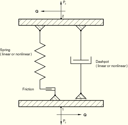
Figure 1: Spring and Dashpot
1.1. Applications of Abaqus Spring Element
- Modeling Physical Springs: These elements can directly represent physical springs in a mechanical system, where the force-displacement relationship is crucial.
- Axial or Torsional Components: Idealize components that behave similarly to springs in axial or torsional modes.
- Structural Dampers: By specifying structural damping factors, spring elements can model dampers, contributing to the imaginary part of the spring stiffness.
- Rigid Body Motion Restraints: Prevent or limit rigid body motion in mechanical assemblies.
- Frequency-Dependent Analysis: Suitable for direct-solution steady-state dynamic analysis where spring stiffness can depend on frequency.
2. Different behaviors of spring element
There are two types of behavior: Linear and Nonlinear. Let’s define each one.
Linear Behavior
Definition: Linear behavior in spring elements is characterized by a constant spring stiffness, meaning the force-displacement relationship is proportional and described by Hooke’s Law.
Characteristics:
- The stiffness can be dependent on temperature and field variables.
- For direct-solution steady-state dynamic analysis, the stiffness can also depend on frequency.
Formula:
![]()
where F is the force, K is the spring stiffness, and Δu is the relative displacement.
Nonlinear Behavior
Definition: Nonlinear behavior is defined by pairs of force-relative displacement values, allowing the spring to exhibit non-proportional stiffness characteristics. Nonlinear springs have a variable stiffness that changes with displacement. This behavior is more representative of real-world springs, especially under large deformations.
Characteristics:
- The force remains constant outside the provided range of displacement values.
- Nonlinear behavior can also be dependent on temperature and field variables.
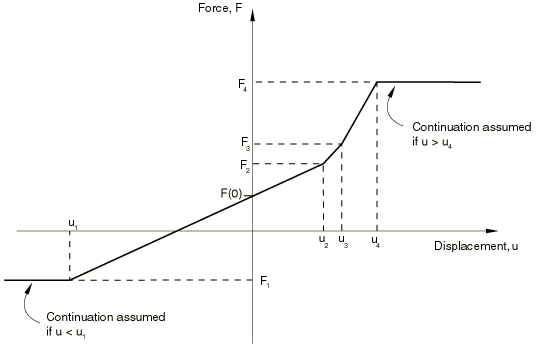
Figure 2: Nonlinear spring [reference]
Complex Stiffness
Definition: Complex stiffness is used to simulate structural dampers. It includes both a real part (stiffness) and an imaginary part (damping factor).
Characteristics:
- The structural damping factor s contributes to the imaginary part of the stiffness.
- The imaginary part of the stiffness is calculated as “isK”, where i is the imaginary unit.
- These data can be frequency-dependent.
Formula:
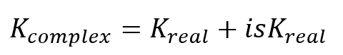
where Kreal is the real part of the spring stiffness and s is the structural damping factor.
Speaking of Damping; you know you can learn about damping and how to apply it in contacts in Abaqus by reading this article: What is Abaqus Contact Damping and how to apply it in Abaqus?
3. Types of Abaqus spring element
There are three types of Abaqus spring element: SPRING1, SPRING2, and SPRINGA.
The SPRING1 and SPRING2 elements are exclusive to Abaqus/Standard. SPRING1 connects a node to the ground and operates in a fixed direction, while SPRING2 connects two nodes and also operates in a fixed direction.
The SPRINGA element is available in both Abaqus/Standard and Abaqus/Explicit. SPRINGA connects two nodes and its line of action follows the line connecting these nodes, allowing it to rotate during large-displacement analysis.
All spring elements in Abaqus, including SPRING1, SPRING2, and SPRINGA, can exhibit either linear or nonlinear behavior.
SPRING1 and SPRING2 can be linked to either displacement or rotational degrees of freedom (as torsional springs in the latter case). However, using torsional springs in large-displacement analysis requires careful definition of total rotation at a node. Therefore, connector elements are typically a more suitable option for providing torsional springs in large-displacement scenarios.
SPRINGA
Description: An axial spring between two nodes, with its line of action being the line joining the two nodes. This line of action may rotate in a large-displacement analysis.
Nodal Coordinates Required: X, Y, Z coordinates are necessary for calculating the action of the element.
Element Output:
- S11: Force in the spring.
- E11: Relative displacement across the spring.
SPRING1
Description: A spring between a node and ground, acting in a fixed direction.
Nodal Coordinates Required: None. The element nodes do not need to have coordinates defined as the action associated with these elements is defined by specifying the degrees of freedom involved.
Element Output:
- S11: Force in the spring.
- E11: Relative displacement across the spring.
SPRING2
Description: A spring between two nodes, acting in a fixed direction.
Nodal Coordinates Required: None. Similar to SPRING1, the element nodes do not need to have coordinates defined.
Element Output:
- S11: Force in the spring.
- E11: Relative displacement across the spring.
4. Abaqus Spring Element Degrees of Freedom
SPRINGA
Active Degrees of Freedom:
1, 2, 3.
The translational degree of freedom in the 3-direction is not activated in an Abaqus/Standard analysis if both nodes of the element are connected to two-dimensional entities such as two-dimensional analytical rigid surfaces, two-dimensional beam elements, etc.
SPRING1 and SPRING2
Active Degrees of Freedom:
1, 2, 3, 4, 5, or 6.
If you specify a local orientation for the spring, these are local degrees of freedom. Otherwise, these are global degrees of freedom.
5. Modeling different stiffnesses in compression and tension (Spring Stiffness Abaqus)
How can I model a spring element in Abaqus, which has a different stiffness in compression from that in tension (spring stiffness Abaqus)?
As you may know, we can define a spring element between two points by using the Special menu in the Interaction module to define Springs/Dashpots features:
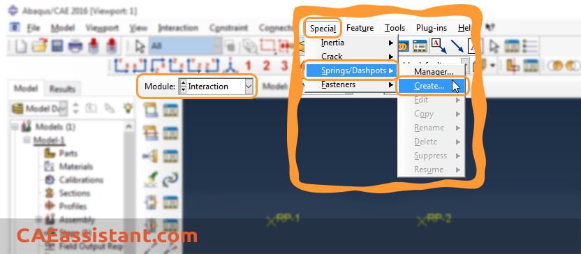 (Here, to have a very simple model, we have defined two Reference Point in Assembly module before.)
In Edit Springs/Dashpots window that appeared after selecting two points, you can define spring stiffness:
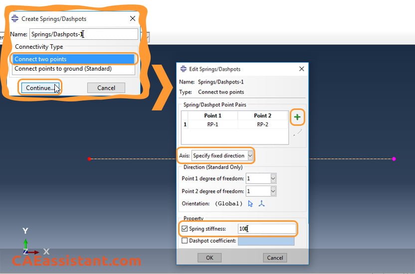 This stiffness will be same for tension and compression. If you want to define different tensile and compressing stiffness, you must bother yourself more using Abaqus Keywords editor:

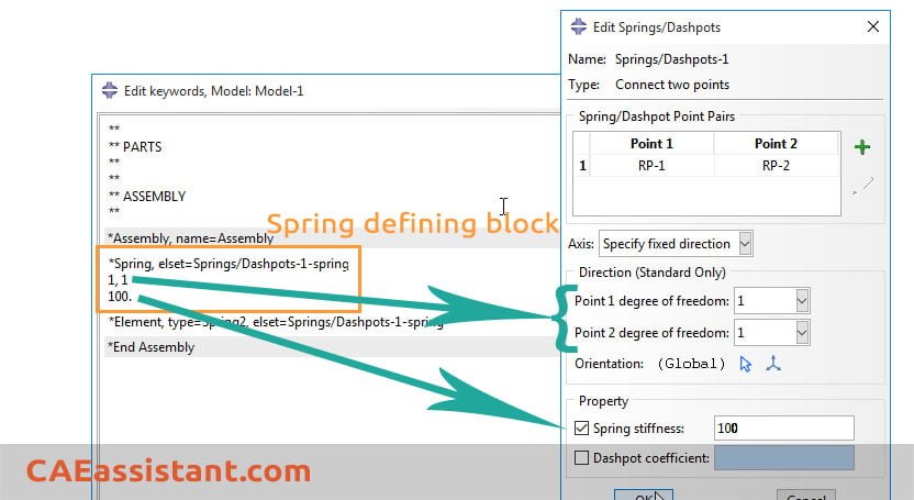 Now, you can see the keywords created by Abaqus automatically due to graphical commands in Abaqus/CAE when creating the spring:
By adding the nonlinear term in the spring definition block (*Spring keyword) one could then define Spring behavior which is different for compression and tension. Just click on the *Spring… line and edit the block as below:
(When you start editing, the color of affected block will turn into pink)
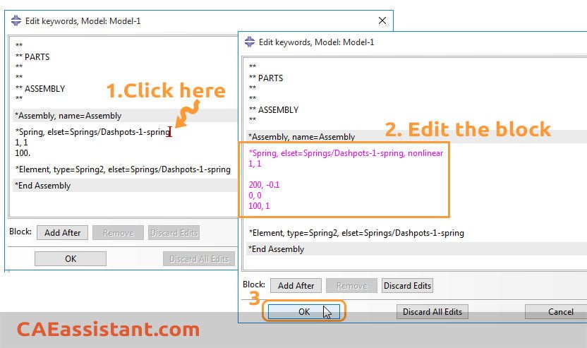 The data line added are:
Force1, Displacement-1
0.0, 0.0
Force3, Displacement-3
This new block means that when you apply -1.0 m displacement, the spring will create 200 N force, so K=F/x=200/1=200 N/m. This is the stiffness in compression. Then you define tensile stiffness by saying 1.0 m displacement for 100 N force. This is K=100 N/m (as before).
6. Conclusion
In conclusion, Abaqus Spring Elements are essential tools for simulating the behavior of mechanical systems with precision and versatility. These elements enable the accurate modeling of physical springs, axial and torsional components, and structural dampers, accommodating both linear and nonlinear behaviors. They can be tailored to depend on temperature, field variables, and frequency, enhancing their applicability across various engineering scenarios.
We explored the different types of Abaqus Spring Elements, including SPRING1, SPRING2, and SPRINGA, each with unique features suited for specific analysis needs. The linear behavior, defined by constant stiffness, and the nonlinear behavior, characterized by variable stiffness, were thoroughly examined. Additionally, we discussed how to model springs with different stiffnesses in compression and tension using the Abaqus Keywords editor.