

Frustrated by Abaqus errors? Explore our comprehensive guide covering 14 essential techniques for finding Abaqus errors and solutions to master your simulations. From unit checks to output analysis and thorough Abaqus Datacheck, we’ve got you covered. Don’t let errors in Abaqus hold you back – Stay with CAE Assistant!
1. Debugging Errors in Abaqus | Convergence Meaning
As it defines itself, Bug means anything annoyance that causes your problem not to be solved or without accurate results. debugging means any actions that need to be done to solve a problem correctly, without any errors, and obtain accurate results.
Convergence is a term to say our problems equations and matrices are solved properly to have our job completed even without any warnings. But, are the results accurate and according to the actual model? If not, then you have to start debugging. You could say that convergence is a subset of the debugging process.
Now, let’s debug the ABAQUS errors with some techniques.
Read More: Abaqus tutorial video & PDF
2. Debugging techniques
Here, we introduce some techniques and procedures for debugging ABAQUS errors. Some of them are preprocessing, and some are post-processing:
- System of units check
- Making a test model
- Output check
- Syntax check
- Data check
- Boundary conditions and loadings
- Materials check
- Constraints check
- Elements check
- Interference fits check
- Contact check
- Over Constraints and initial rigid body motion check
- Static stabilization
- Dynamics check
This Abaqus Error list, or, better yet, these debugging techniques, provides valuable clues for troubleshooting and resolving simulation issues. Let’s explore them.
 |
⭐⭐⭐ Abaqus Course | ⏰10 hours Video 👩🎓+1000 Students ♾️ Lifetime Access
✅ Module by Module Training ✅ Standard/Explicit Analyses Tutorial ✅ Subroutines (UMAT) Training … ✅ Python Scripting Lesson & Examples |
2.1. System of Units Check
In the first step of debugging process, you should check the units of your input data to see if they are consistent or not. After that, you should review the boundary conditions and loading to ensure there aren’t any issues. For more information about the system of units, click here.
It’s worth mentioning that sometimes inconsistent units may not cause any issues or errors in Abaqus. However, it’s crucial to have a sense of the scale of the results.
2.2. Creating a Test Model to Minimize Abaqus Errors
A large model may take a long time to be analyzed, so making a test model speed up the debugging process is highly recommended. The test model is simplified and miniaturized from the original model created for speeding up the debugging process. It should be only used for debugging and testing.
2.3. Output Check
Having more information about your problem before or after submitting a job is always useful. However, for debugging purposes, request more results through the “Field Output” and “History Output” in the Step module (see figures 1 and 2) to debug the analysis afterward. Obviously, it will take more computational time, but it is worth it because these requests will help you debug the system and find the convergence issues.
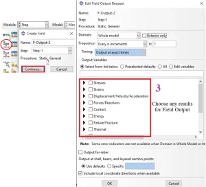
Figure-1 Field Output requests
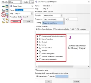
Figure-2 History Output requests
2.4. Syntax Check
When you want to check your input file to see any flaws in your script, you should use the syntax check command. It checks your input file line by line, and finds and shows any flaws that may exist in the file’s script. After a syntax check, check the “.log” file, and if there are no flaws, you will see the lines as shown in figure 3. To do a syntax check, type the command line “abq6142 syntaxcheck j=your input file’s name” in a command prompt window. For more information, click here.
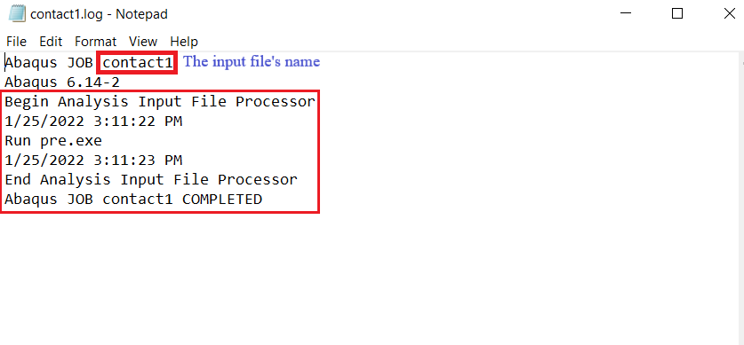
Figure 3 The input file without flaws
Now, let’s move on to the next one, ‘Abaqus Datacheck.’ Mastering the understanding of this tool could greatly benefit us.
2.5. Abaqus DataCheck
The data check is the same as the syntax check with one difference; the data check runs the file to ensure that the model has all the required options. It checks the model consistency as well. You could say the syntax check is the subset of the data check.
The procedure to execute a Abaqus datacheck is the same as the syntax check, with only a slight difference in the command line:
abq6142 datacheck j=your input file’s name
The log file message is different (see figure 4). Also, you could use the data check through the GUI (see figure 5).
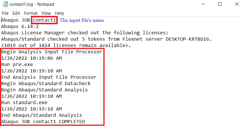
Figure-4 The log file without error
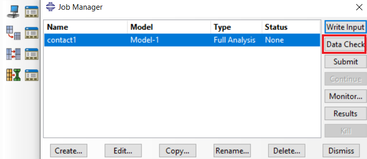
Figure-5 Data check through the GUI
As mentioned, mastering Abaqus Datacheck and Syntax Check can be immensely helpful during troubleshooting. To become proficient in these, you simply need to practice with various examples, such as writing subroutines, Python scripting, or more common projects. You can join our free course to explore different Abaqus examples.
2.6. Boundary Conditions and Loading
After a syntax and data check, you can correctly run the model’s input data into the ABAQUS. Moreover, you can ensure that appropriate settings are applied according to the model specifications. After that, check the boundary conditions and loading. You must monitor them to ensure that the applied boundaries and load cases have appropriate settings with proper ABAQUS features.
2.7. Materials Check
Check the material properties. You must check them to ensure that the model’s structural responses present proper behavior under the boundary conditions and loading. Also, apply physical behavior law and material data’s complexity function to the model.
2.8. Constraints Check
If you have to use constraints (see figure 6), make sure to use the right one according to your problem. For example, when you need to couple the motion of a surface or a group of nodes to a reference node, you must use “Couple constraint.” There are two based methods for the Couple: Kinematic and distributing. You must choose the proper method according to the problem. 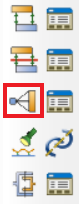
Figure 6 Constraint option
2.9. Elements Check
Sometimes the elements cause numerical difficulties in the model, such as: selecting the wrong element type, improper meshing, hourglass control, not using Hybrid elements in the incompressible models, etc. Therefore, you must check the elements to debug your model.
The next item to check is “Interference Fits,” which can be particularly helpful in specific scenarios. Remember, this is just one aspect of the “Abaqus errors and solutions” procedure. It’s essential to try all these techniques to effectively debug your projects.
2.10. Interference Fits Check
This part is about using contact to solve interference problems by focusing on interference fits. The interference means excessive overclosure between surfaces. An interference fit (press fit, friction fit) is a method to fasten two parts by pushing them together with normal force, and they get stuck together by friction rather than any means of fastening. A typical example is shaft press-fitting into bearings. You can resolve the interference problems in surface-to-surface contact for the ABAQUS/Standard. Select the desired step and use the interference fit option (see figures 7 and 8).
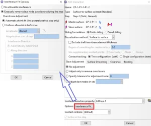
Figure-7 The interference fits option through the GUI
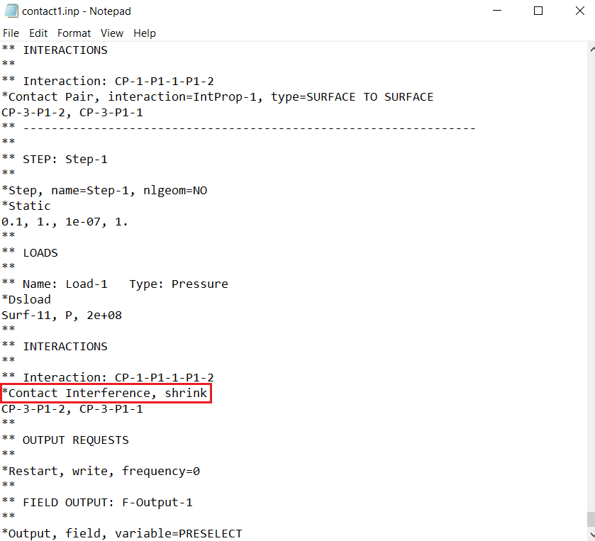
Figure-8 The interference fits option through the input file
2.11. Contact Check
It is relatively easy to define contact interactions. However, adding local contact stiffness can cause instability problems in the global stiffness matrix and make the matrix nonsymmetric. So, several numerical difficulties may occur. One of the good methods to prevent these issues is to select the master and slave surface correctly. The master surface should be rigid or with a higher Young’s module. Also, the master surface should have a coarser mesh than the slave surface.
2.12. Over Constraints and Initial Rigid Body Motion Check
In an analysis, one reason for convergence issues is inadequate or improper boundary conditions. Also, a model can be under or over-constrained, leading to convergence issues. If you do not use enough boundary conditions, your model may move as a rigid body in any direction (rigid body motion). The rigid body motion causes the stiffness matrix to become singular. As a result, the ABAQUS will show “zero pivot” warning messages. Although the software tries to solve the issue, it’s not always working. Therefore, you have to check the warnings and fix the constraints and boundary conditions.
It’s possible that you have considered all the previous techniques, but your project doesn’t converge, and you still face an error in Abaqus. The next technique is helpful for those encountering convergence errors.
2.13. Static Stabilization Check
The ABAQUS finite element software uses this main equation to solve a problem:
“K” is the stiffness matrix, “x” is the displacement matrix, and “F” is the Force matrix. Whenever a static problem becomes unstable, the equation cannot solve the problem because of the numerical difficulties caused by instability in the model. So, a damping force component will be added to the equation so that the problem can be solved:
![]()
“D” is the damping coefficient that stabilizes the problem and makes a quasi-static solution. Therefore, the “D” value must be controlled to get as nearly static a solution as possible. To do so, compare the ALLSD and ALLIE energies levels. For more information, click here.
2.14. Dynamics Check
In static analysis, there is no effect of damping or mass (inertia). The applied load acts fully immediately on the model instead of with time increment because it has no physical sense. On the other hand, the dynamic analysis has a physical sense regarding applied load versus time. Moreover, the effect of mass and damping are included as well. The static analysis uses an Implicit solver. The dynamic analysis can use the Explicit solver or the Implicit. When you have a dynamic problem, you need to check which solver is appropriate for the analysis, Implicit or Explicit. Learn more.
Exploring this “Abaqus Errors and Solutions” article is crucial for enhancing your simulation troubleshooting skills. It’s important to note that in this article, we’ve provided an introduction to each technique. To effectively address ABAQUS errors and gain a deeper understanding of these techniques, we encourage you to enroll in CAE Assistant free course, where you can apply these techniques to a variety of Abaqus examples.
Please share your views with us in the comment section. We really appreciate your feedback, as it helps us improve our tutorials and fulfill all your CAE needs without requiring additional tutorials. Our primary reference for writing this article is the Abaqus documentation. You can also access the PDF version of this post by clicking on “Abaqus Errors and Solutions.”
|
⭐⭐⭐ Abaqus Course | ⏰10 hours Video 👩🎓+1000 Students ♾️ Lifetime Access
✅ Module by Module Training ✅ Standard/Explicit Analyses Tutorial ✅ Subroutines (UMAT) Training … ✅ Python Scripting Lesson & Examples |
Frequent asked questions
What are the top 10 techniques for debugging errors in Abaqus?
- System of units check: Verify input data for consistency in units.
- Test model creation: Speed up debugging by using smaller test models.
- Output check: Request additional results for analysis in the Step module.
- Syntax and data check: Examine your input file for script errors.
- Boundary conditions and loadings: Confirm settings are appropriate.
- Materials check: Ensure structural responses match expected behavior.
- Constraints check: Select the right constraints for your problem.
- Elements check: Address numerical difficulties caused by elements.
- Interference fits check: Use contact to resolve interference issues.
| ✅ Subscribed students | +80,000 |
| ✅ Upcoming courses | +300 |
| ✅ Tutorial hours | +300 |
| ✅ Tutorial packages | +100 |
This article is one of the most useful articles for Abaqus. I was able to solve many of the errors I encountered in Abaqus.