
Linear velocity refers to how fast an object moves in a straight line, while angular velocity measures the rate of rotation around an axis. Linear velocity is measured in units such as meters per second (m/s), whereas angular velocity is measured in radians per second (rad/s). The main difference is that linear velocity focuses on straight-line movement, while angular velocity describes rotational motion. In this blog, we will also explore how to apply these concepts in Abaqus using “Abaqus Velocity” and discuss “Angular Velocity VS Linear Velocity” to provide a clear understanding of their practical applications.
Tangential velocity, on the other hand, is the linear speed of an object moving along a circular path, measured at any point tangent to the circle. It differs from angular velocity in that tangential velocity considers the actual speed of a point on the rotating object, while angular velocity measures the rate of rotation. By understanding these distinctions, we can effectively analyze and design mechanical systems in various fields.
1. What is Linear velocity?
Linear velocity refers to the rate of change of an object’s position with respect to time in a straight line. In simpler terms, it measures how fast something is moving in a particular direction.
1.1. Examples of Linear Velocity in Real Life
- Car on a Highway: When a car travels at a constant speed of 60 miles per hour on a straight road, it has a linear velocity.
- Runner on a Track: A sprinter running 100 meters in 10 seconds has a linear velocity calculated as the distance divided by the time.
- Airplane Taking Off: An airplane accelerating down the runway before takeoff demonstrates increasing linear velocity.
1.2. Unit and Formula of Linear Velocity
Unit
The standard unit for linear velocity is meters per second (m/s). However, it can also be expressed in other units such as kilometers per hour (km/h) or miles per hour (mph).
Formula
The formula to calculate linear velocity V is:
V=td
where:
- V is the linear velocity,
- d is the distance traveled,
- t is the time taken.
If a cyclist travels 120 meters in 20 seconds, the linear velocity can be calculated as follows:
V = 120/20 = 6 m/s
1.3. Types of Linear Velocity
- Uniform Velocity
Uniform velocity occurs when an object travels in a straight line at a constant speed. This means both the magnitude and direction of the velocity remain unchanged over time.
Example: A car cruising on a straight highway at a constant speed of 80 km/h.
- Non-Uniform Velocity
Non-uniform velocity occurs when either the speed or direction (or both) of the object changes over time. This indicates acceleration or deceleration in linear motion.
Example: A car slowing down as it approaches a red light, where the speed decreases over time.
- Relative Velocity
Relative velocity is the velocity of one object as observed from another moving object. It helps in understanding the motion of objects with respect to each other.
Example: If two cars are moving on a highway, one at 70 km/h and the other at 50 km/h, the relative velocity of the first car with respect to the second car is 20 km/h.
1.4. Understanding Linear Velocity and its Role in Motion and Kinematics
Linear velocity is a fundamental concept in kinematics, the branch of physics that describes motion. Understanding linear velocity allows us to:
Predict Motion: By knowing an object’s velocity, we can predict where it will be at a future point in time.
Analyze Forces: Velocity helps in analyzing the forces acting on an object. For instance, changes in velocity indicate the presence of acceleration, which is caused by forces according to Newton’s second law.
Design Systems: Engineers use linear velocity to design systems like transportation networks, conveyor belts, and amusement park rides, ensuring they operate efficiently and safely.
2. What is Angular Velocity?
Angular velocity is a measure of the rate of rotation around an axis. It tells us how fast something is spinning or rotating and the direction of the rotation.
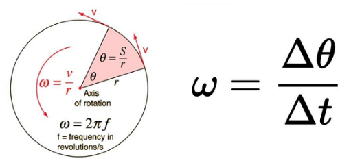
Figure 1: Angular velocity
2.1. Real-Life Examples of Angular Velocity
- Earth’s Rotation: The Earth rotates about its axis once every 24 hours. This rotational movement can be described by its angular velocity.
- Wheels of a Car: When a car moves, its wheels spin. The speed of this spinning is an example of angular velocity.
- Fan Blades: The blades of a ceiling fan rotate around a central point, and the speed of this rotation is another instance of angular velocity.
2.2. Unit and Formula
- Angular velocity is symbolized by the Greek letter omega (ω).
- The SI unit is radians per second (rad/s).
- It’s calculated using the formula: ω = Δθ / Δt
- Δθ (delta theta) represents the angular displacement (change in angle) in radians.
- Δt (delta t) represents the time interval in seconds.
2.3. Example Calculation
If a record player completes one full rotation (360°) in 5 seconds, what’s its angular velocity?
- Convert degrees to radians: 360° * (π / 180°) = 2π radians (since a full circle is 2π radians)
- Apply the formula: ω = 2π radians / 5 seconds = 0.4π rad/s
2.4. Types of Angular Velocity
- Rotational Velocity: This is the most common type, referring to the spinning of an object about a fixed axis (like the merry-go-round).
- Spin Angular Velocity: This describes the rotation of an object about its own center of mass (like the Earth spinning).
- Orbital Angular Velocity: This refers to the rotation of an object around another fixed point (like the Earth orbiting the Sun).
2.5. Role of Angular Velocity in Motion and Kinematics
Angular velocity plays a critical role in the study of rotational motion and kinematics. Here’s how it influences and interacts with various aspects of motion and kinematics:
Describing Rotational Motion: Angular velocity provides a quantitative measure of how fast an object is rotating. It is essential for describing the rotational state of objects in systems ranging from simple wheels to complex machinery.
Relationship with Linear Velocity: In circular motion, linear velocity (the speed along the circular path) is directly related to angular velocity through the radius of the circle. This relationship helps in understanding the dynamics of objects in circular motion. The formula linking them is:
V = r⋅ω
where v is the linear velocity, r is the radius, and ω is the angular velocity.
Kinematic Equations for Rotational Motion: Just like linear motion, rotational motion can be described using kinematic equations. Angular velocity, angular acceleration, and angular displacement are used to predict and analyze rotational motion. The basic kinematic equations for rotational motion include:
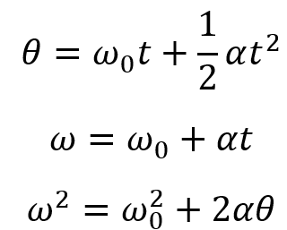
where θ is the angular displacement, ω0 is the initial angular velocity, ω is the final angular velocity, α is the angular acceleration, and t is the time.
Centripetal Force and Acceleration: In any rotational system, the objects experience centripetal acceleration directed towards the center of the rotation. This is given by:
![]()
where ![]() is the centripetal acceleration. Understanding this concept is crucial for analyzing forces in rotational systems, such as in the case of a car turning around a curve.
is the centripetal acceleration. Understanding this concept is crucial for analyzing forces in rotational systems, such as in the case of a car turning around a curve.
Angular Momentum and Torque: Angular velocity is integral to concepts like angular momentum (L=Iω) and torque (τ=Iα), where I is the moment of inertia. These concepts are fundamental in rotational dynamics, helping to understand the effects of forces and the conservation of angular momentum in systems.
Applications in Engineering and Physics: Angular velocity is critical in designing and analyzing the performance of mechanical systems such as gears, turbines, and engines. In physics, it helps in understanding the behavior of celestial bodies, gyroscopes, and rotating systems.
3. What is tangential velocity?
Tangential velocity is the instantaneous linear speed of an object moving along a circular path, measured at any point tangent to the circle. This velocity is always directed along the tangent to the circle at the point of interest.
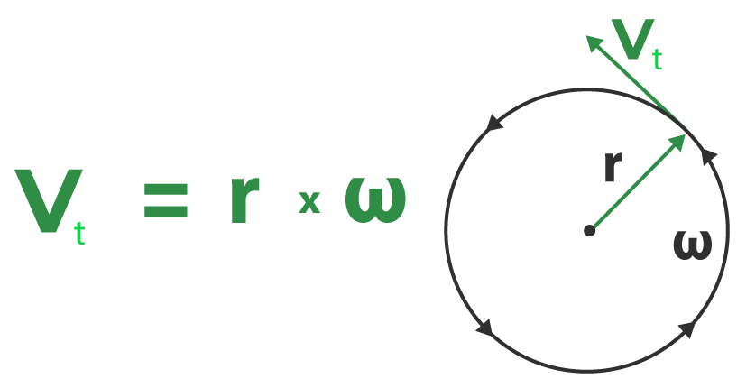
Figure 2: Tangential velocity [2]
3.1. Real-life examples
- Car Wheels: As a car drives, the tangential velocity of any point on the wheel is the speed at which that point would move in a straight line if it were to leave the wheel.
- Amusement Park Rides: For rides like a Ferris wheel, the tangential velocity is the speed at which seats are moving along the circular path.
- Earth’s Rotation: Points on the equator have higher tangential velocity than points closer to the poles due to Earth’s rotation.
3.2. Formula and Units
The formula for tangential velocity (Vt) is given by:
![]()
where:
- Vt is the tangential velocity,
- r is the radius of the circular path,
- ω is the angular velocity.
The unit of tangential velocity is meters per second (m/s).
3.3. Calculation Example
Consider a disc with a radius of 0.33 meters rotating at an angular velocity of 15 radians per second. To find the tangential velocity:
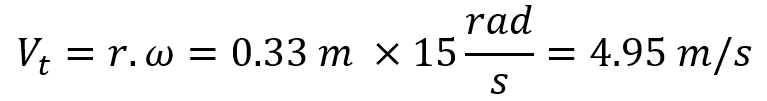
3.4. Role in Motion and Kinematics
Describing Motion: Tangential velocity provides a clear understanding of how fast and in what direction a point on a rotating object is moving.
- Relating Linear and Angular Quantities: It connects linear motion and angular motion, showing the relationship between an object’s speed along the edge of a circle and its rate of rotation.
- Centripetal Force Calculation: Understanding tangential velocity is crucial for calculating the centripetal force required to keep objects in circular paths.
- Applications in Engineering: Engineers rely on the concept of tangential velocity to design and analyze mechanical systems involving rotational components, such as gears and turbines.
4. Angular Velocity VS Linear Velocity
Angular velocity measures how fast an object rotates, while linear velocity measures how fast an object moves in a straight line.
The key relationship between them is:
![]()
where v is the linear velocity, r is the radius, and ω is the angular velocity.
Some key points:
- Angular velocity is measured in radians/second, while linear velocity is measured in distance/time units like m/s.
- For circular motion, the linear velocity is tangent to the circle at any point.
- Angular velocity remains constant for all points on a rigid rotating object, while linear velocity increases with distance from the axis of rotation.
4.1. Conversion Factors and Common Units
- Radians and Revolutions: One revolution is equal to 2π radians. So, to convert from revolutions per minute (RPM) to radians per second (rad/s), multiply by 2π/60.
- Distance Units: One mile is equal to 5,280 feet, and one kilometer is equal to 1,000 meters. These conversions are useful when dealing with different units of measurement.
4.2. Example
A disc with a radius of 4 centimeters spins at 30 revolutions per minute. What is the linear speed in feet per second?
- Convert RPM to radians per second:
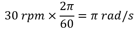
2. Use the formula:
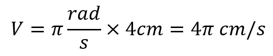
3. Convert centimeters to feet (1 meter = 3.281 feet, 1 meter = 100 centimeters):

5. Tangential Velocity VS Angular Velocity
Tangential velocity (𝑣𝑡) and angular velocity (𝜔) are related through the radius (r) of the circular path on which an object is moving. The tangential velocity is the linear speed of an object moving along the circular path, while the angular velocity is the rate at which the object sweeps out an angle around the center of the circle.
Angular velocity and tangential velocity are two ways to describe the motion of a rotating object, but they capture different aspects of that motion. Here’s a breakdown:
Angular Velocity (ω):
- Focuses on the rotation itself.
- Tells you how fast an object is spinning in terms of angular displacement (measured in radians) per unit time (seconds).
- Units: radians per second (rad/s).
- Same for all points on a rigidly rotating object.
Tangential Velocity (Vt):
- Focuses on the linear speed of a specific point on the rotating object.
- Represents the actual speed of that point as it travels along a circular path.
- Units: meters per second (m/s) or any other unit of linear speed.
- Varies depending on the distance of the point from the axis of rotation. Higher distance from the axis leads to higher tangential velocity.
5.1. Relation between them
They are related by the following equation:
Vt = ω * r
where:
- Vt is the tangential velocity
- ω is the angular velocity
- r is the distance between the point and the axis of rotation (radius)
5.2. Converting between them
To find tangential velocity (Vt) of a point, you need to know the angular velocity (ω) and the distance (r) from that point to the axis of rotation. Just plug those values into the formula above.
To find angular velocity (ω) from tangential velocity (Vt) and distance (r), you can rearrange the formula: ω = Vt / r
5.3. Example
Imagine a merry-go-round rotating at 2 rad/s. A child sits 3 meters from the center.
What’s the tangential velocity of the child?
Vt = ω * r = 2 rad/s * 3 m = 6 m/s (The child travels 6 meters every second along the circular path)
If another child sits 2 meters from the center, what’s their tangential velocity?
Vt = ω * r = 2 rad/s * 2 m = 4 m/s (As expected, the closer child has a lower tangential velocity)
6. How to apply Abaqus Velocity and angular velocity?
Velocity and angular velocity can be specified in Abaqus as initial conditions or boundary conditions. Here’s how to do it:
As Initial Conditions:
Go to Load module > Click on “Create Predefined Field” > Select “Initial” step > “Mechanical” category > select “Velocity” type
Choose the region (part or assembly) where you want to apply the initial velocity. Next, from the Definition combo box, choose one of the options “Translational only”, “Rotational only”, or “Translational & rotational” to select velocity, angular velocity, or both of them, respectively.
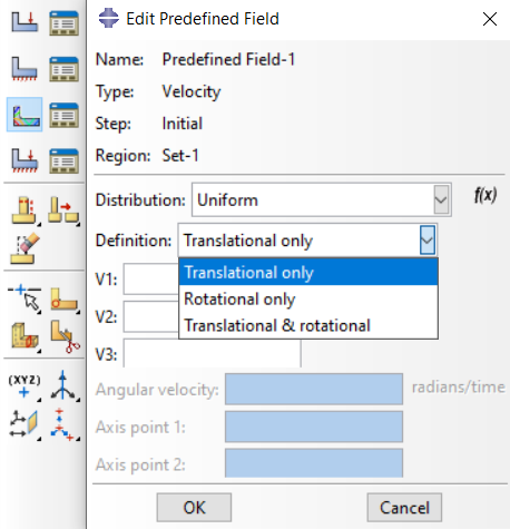
Figure 3: Abaqus velocity as initial conditions
As Boundary Conditions:
Go to Load module > Click on “Create Boundary Conditions” > Select the step in which you want to apply the boundary condition > “Mechanical” category > select “Velocity/Angular velocity” type
Choose the region (part or assembly) where the velocity boundary condition will be applied.
Specify the velocity components in the appropriate fields.
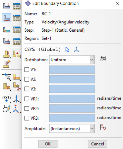
Figure 4: Abaqus velocity as boundary conditions
7. Some issues in applying Abaqus Velocity / Angular velocity
I attempted to simulate external turning using Abaqus, with the workpiece speed set to 6.28/s and the analysis step time set to 1. The workpiece should theoretically revolve one revolution, but the output shows that the workpiece reference point did rotate one revolution, but the rotation involved in cutting appears to be minor.
1. The accompanying figure 1 depicts the workpiece’s boundary conditions (figure 2 shows the workpiece reference point is coupled to the left cross-section.).
2. The output rotation angle of the reference point on the workpiece is shown in figure 3.
- The cloud diagrams 4&5 below illustrate how little the workpiece actually rotates.
How do I adjust the rotation boundary conditions so that the part’s real rotation matches the settings in the Abaqus cutting simulation?
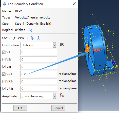 Figure 1
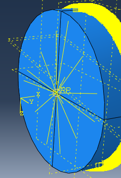
Figure 2
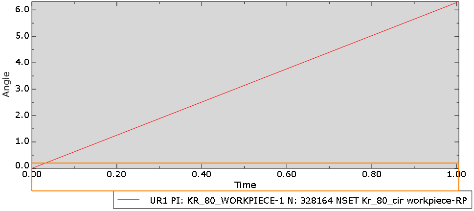 Figure 3
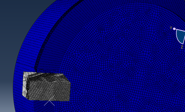 Figure 4
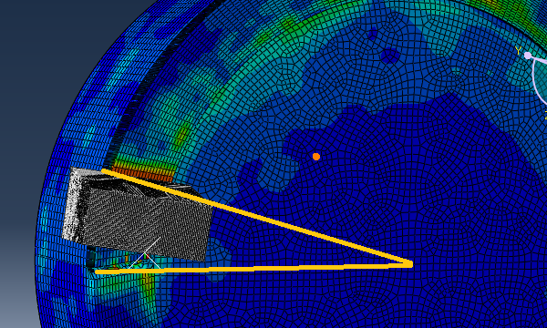 Figure 5
Hello,
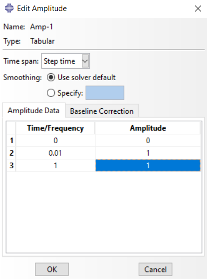
You just need to create an Amplitude for your boundary conditions. Your velocity needs to be continuous. You see, your current boundary condition has no amplitude, and the angular velocity you specified will be applied instantaneously. It’s like applying initial velocity, so if the part makes contact with an object like the tool, this slows down the rotational speed. That is why it rotates with a small amount in the cutting process.
Therefore, create an amplitude. For example, see the figure I attached.
Also, I suggest checking the link below. It will give you useful information to resolve your future problems.
ABAQUS course for beginners | FEM simulation tutorial
Best wishes.
8. Conclusion
In conclusion, understanding the concepts of linear velocity, angular velocity, and tangential velocity is essential for analyzing motion in both straight and rotational contexts. Linear velocity describes how fast an object moves in a straight line, while angular velocity focuses on the rate of rotation around an axis. Tangential velocity bridges the two by explaining the linear speed of an object moving along a circular path.
In practical applications, particularly in engineering and physics, these concepts help in designing and analyzing systems effectively. Using “Abaqus Velocity” to specify these conditions in simulations further aids in predicting and optimizing system performance. By comparing “Angular Velocity VS Linear Velocity,” we gain insights into different aspects of motion, enabling us to tackle real-world problems more efficiently.