


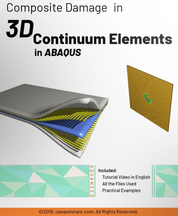
Simulation of composite Hashin damage in 3d continuum element in Abaqus (UMAT-VUMAT-USDFLD)
In this training package, the 3D continuum HASHIN damage initiation model is prepared via three subroutines (USDFLD, UMAT and VUMAT). UMAT Hashin
There is no damage model for the continuum elements in Abaqus software. Thus, we need to use subroutine writing in Abaqus. Note that each subroutine presented in this training package has a different function. USDFLD subroutine does not need to fill the equations to form the stiffness matrix, and the property reduction is applied based on the information that the equations are placed in the subroutine according to the theory of failure. UMAT Hashin subroutine is used for damage when we have to use a standard solver like static-general, soil and etc. Also, the VUMAT subroutine helps us perform damage analysis in cases with dynamic analysis and non-linear problems and convergence problems.
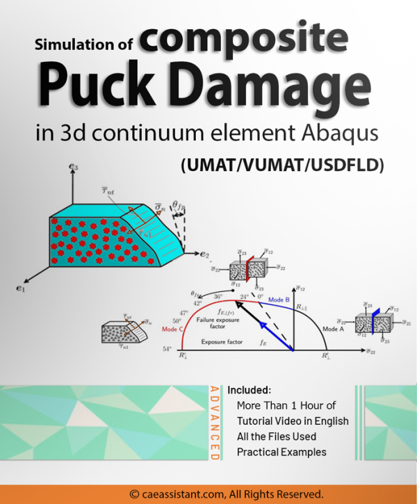
This training package teaches you subroutines line-by-line. It should be noted that after damage initiation, failure occurs suddenly and in the form of a reduction in properties in the model. The HASHIN theory for this package is based on Kermanidis article titled” FINITE ELEMENT MODELING OF DAMAGE ACCUMULATION IN BOLTED COMPOSITE JOINTS UNDER INCREMENTAL TENSILE LOADING. “ The following failure modes are checked in this failure criterion. As mentioned before, the material properties degradation is applied based on the failure mode. UMAT Hashin 3d is discussed there.
1- Matrix tensile failure
2. Matrix compressive failure
3-Fiber tensile failure
4. Fiber compressive failure
5-Fiber-matrix shear-out
6-Delamination in tension and Delamination in compression
You can access all subroutine and software files immediately after purchase on your dashboard. Then, the video training will be available on your dashboard with delay. UMAT Hashin, VUMAT Hashin, and USDFLD Hashin subroutine writing training videos would be unique.
Workshop-1 part-1:Simulation of composite Hashin damage in 3d continuum element in Abaqus with UMAT
After explaining the UMAT subroutine line by line, we enter the Abaqus software and do all necessary settings in the GUI: creating a simple 3D plate, doing the required settings in the Property module and creating composite layup, creating Step, selecting the required outputs. Next, we create four models for the UMAT subroutine. The difference between them is in the boundary conditions and loading; the two models will be under the compression state, and the loads are applied to the model in the fiber and matrix directions. The other two will be in a tension state, and the loads will be applied in the fiber and matrix directions.
To verify the results of these four models, we will create four other models with only the Abaqus CAE and use the Abaqus Standard solver. The HASHIN damage will be modeled in shell elements in all four models; because, as you know, the HASHIN damage is available only on shell and continuum shell elements in the Abaqus CAE. The four models will be under tension and compression in fiber and matrix directions.
First, the VUMAT subroutine will be explained completely. After that, a simple 3D plate will be created, just like the UMAT model. The settings in the Property module would be different, especially when it comes to defining the composite layers; it would be different than the UMAT model. Next, the Explicit solver will be used, and the required outputs will be selected. Like the UMAT model, we will have four models for the VUMAT-HASHIN modeling. Two of them will be under tension loading in fiber and matrix directions. The other two will be under compression loading in fiber and matrix directions.
Like the UMAT models, we would verify these models as well. We will create four models, but we will use the Explicit solver this time. The HASHIN damage will be modeled in shell elements for the same reason. And the four models will be under tension and compression states in fiber and matrix directions.
Like the previous two parts, we first explain the USDFLD subroutine line by line. Then we enter the Abaqus software and model a 3D plate. After that, we apply the proper settings in the Property module, which would be different than the previous two parts. We use the Standard solver, and like the others, we will create four models to cover all types of damage we’ve discussed. Two of them will be under compression in fiber and matrix directions; the other two will be under tension in fiber and matrix directions.
To verify the results, we’re gonna use the same four Standard models that we’ve used for the UMAT.
Summary of the workshop
In this workshop, we wanted to show you how you can model the HASHIN damage in a 3D continuum element with three subroutines; UMAT, USDFLD, and VUMAT.
Each of them has its own advantages and disadvantages for modeling this analysis. Depending on your problem and capability, you can choose one.
We have used the damage criteria mentioned in this article,” FINITE ELEMENT MODELING OF DAMAGE ACCUMULATION IN BOLTED COMPOSITE JOINTS UNDER INCREMENTAL TENSILE LOADING . “ To show you all the types of damage in each subroutine, we had to analyze four models in each of them. Therefore, we would have a total number of 12 models; another four models for verifying the VUMAT subroutine analyzed with Explicit solver and modeled in Abaqus CAE; and four models for verifying the UMAT and USDFLD subroutines. So, when you open the file, you will see 20 models and 20 jobs.
It would be useful to see Abaqus Documentation to understand how it would be hard to start an Abaqus simulation without any Abaqus tutorial. If you are working on Abaqus composite damage and need resources about composite FEM simulation, click on the Abaqus composite analysis page to get more than 20 hours of video training packages of composite materials simulation.
Read More: All about abaqus composite tutorial
mei97 –
Hello. Thank you for preparing this package. it explained all the points and things well. Can other theories be considered in this way? For example, puck theory