Damage Properties of Thermoplastic Polymers with UMAT Subroutine

The goal of this package is to simulate damage properties of thermoplastic polymers with Abaqus using UMAT subroutine.

Lesson 1: Introduction to Thermoplastic Polymers

Thermoplastic polymers are a type of material that can be melted and reshaped multiple times without undergoing chemical changes. They are made up of long chains of repeating units and can be molded when heated and solidified upon cooling. They have various applications in packaging, automotive parts, toys, medical devices, electrical insulation, and textiles. Examples include polyethylene, polypropylene, PVC, polystyrene, and PET.

Thermoplastic polymers have specific behaviors that differ from other materials such as metals. For example, they exhibit significant viscoelasticity, which means their response to an applied load includes both viscous and elastic components. Moreover, thermoplastic polymers often undergo complex deformation mechanisms such as yield, strain hardening, aging, and strain softening. These mechanisms are influenced by factors such as temperature, stress state, and strain rate.
Due to these unique characteristics, specialized models for thermoplastic polymers have a higher level of accuracy compared to general models. These specialized models take into account the specific viscoelastic and deformation behaviors of thermoplastic polymers, allowing for more precise simulations and predictions of their mechanical responses under various loading conditions. In the following, the constitutive model used in this training package is explained.

What is the model used in this package? | Properties of Thermoplastic Polymers

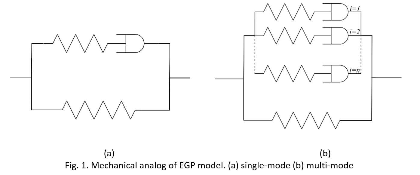
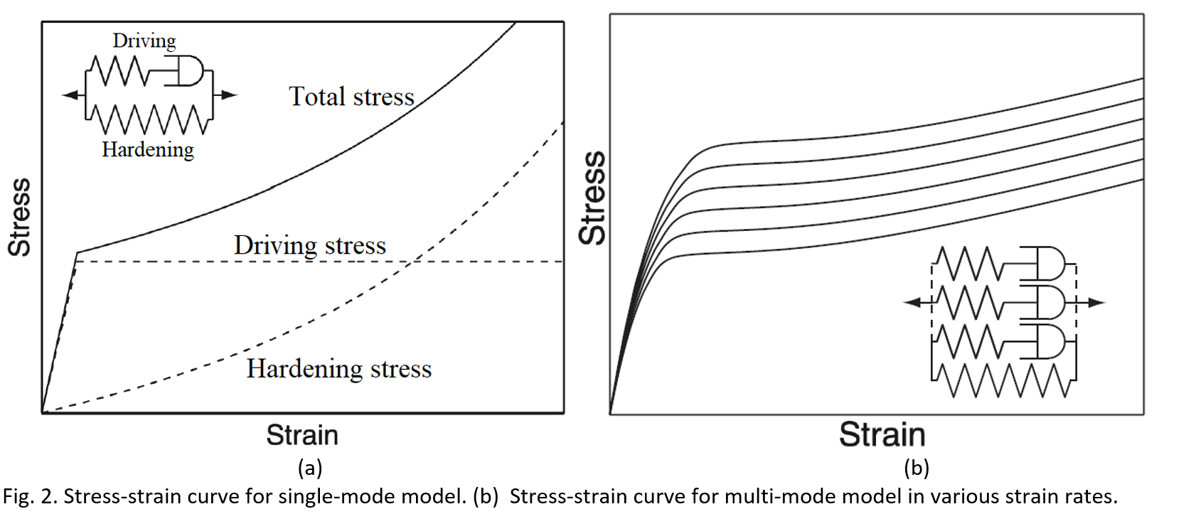
The model used here for the Properties Thermoplastic Polymers is based on the Eindhoven Glassy Polymer (EGP) model (Govaert et al., 1999; Tervoort et al., 1997; Klompen et al., 2005) which is combined with Continuum Damage Mechanics (CDM) to accurately simulate the failure of these material. The EGP model uses two parallel contributions. The first one is the result of the intermolecular interactions of secondary bonds. The second one is the elastic response of the entangled network of the primary bonds, which leads to hardening. The first contribution can be modeled using single or multiple Maxwell branches, known as single-mode and multi-mode models (fig. 1).

Stress Strain Curve for Thermoplastic Polymer

In the multi-mode approach, the nonlinear behavior of the pre-yield regime is captured (figure 2: Stress Strain Curve for Thermoplastic Polymer). The neo-Hookean material model with a non-Newtonian fluid flow rule is used to capture the elasto-viscoplastic deformation in a Maxwell branch. It can accurately capture the mechanical response of polymers by capturing the effect of factors such as strain rate, temperature, thermal history, hydrostatic pressure, and moisture on the material behavior.

To consider the progressive damage in the model and take into account the effects of plastic strain and hydrostatic stress on failure, the damage parameter is introduced to the model using the principle of equivalent strain. The model utilizes the damage evolution law introduced by Lemaitre (2012), which correlates the damage evolution with plastic strain and strain energy. The training provides a more detailed explanation on how to incorporate the damage parameter into the EPG model.

Lesson 2: Theory and Formulation

In this part of the training, the theory and formulation of the model is explained. This section includes four steps to complete the relation between the deformation and stress tensor. In the first step, the kinematics of the model is developed based on large strain theory. The deformation gradient tensor 𝑭 of the driving branch is multiplicatively decomposed to the elastic and plastic parts:

Finally, a new definition of the rate of elastic and plastic deformation  and  are calculated considering this decomposition. Next in the second section, the thermodynamics is used to formulate the relationships between state variables and thermodynamic forces. The Clausius–Duhem inequality states that in a thermodynamic process, the internal dissipation  is always non-negative. In an isothermal case, it can be written as:

where 𝜓 is the free energy potential whereby constitutive equations are derived in the framework of irreversible thermodynamics.

In the third section, the Cauchy stresses are calculated by defining a suitable free energy potential. Assuming that the material is nearly incompressible Neo-Hookean material, the free energy in driving branch  is defined as Bonet and Wood (1997):

where  is the shear modulus for mode 𝑖, and 𝐾 is the bulk modulus. is elastic isochoric right Cauchy–Green deformation tensor of mode i, 𝐷 is the damage parameter, and 𝐽 is the volume ratio which considers the volumetric deformation.

Lesson 3: Numerical Implementation and writing UMAT 

An implicit scheme is used to numerically integrate the constitutive model and implement as a user material subroutine (UMAT) in Abaqus. The general structure of this scheme is such that for a given deformation gradient 𝑭 at the end of a time step, the total stress 𝝈 will be obtained. To do that, the stress in the hardening and the Maxwell branches should be calculated. Hardening stress  and effective hydrostatic stress  can be calculated directly. To calculate the total effective deviatoric driving stresses , the integration has to be carried out iteratively. Since this implicit scheme includes the contribution of all modes, it is called the external scheme here. On the other hand, each mode has to be integrated by an implicit scheme individually called the internal scheme here.

In this training, first, an assumption to simplify implementation is presented. then the internal and external schemes will be discussed. Next, Consistent tangent stiffness matrix is calculated which is needed so that Abaqus can iteratively solve the governing equations with standard implicit solver. Finally, a detailed explanation of how to write the subroutine is provided.

Workshop 1: Simulation of T-fitting Burst Pressure Test 

In this workshop, first, the geometry and test conditions such as the boundary condition and load are explained. Next, the modeling process is explained step by step. Finally, the simulation will be done, and the results will be discussed.

This simulation predicts the failure location in a T-fitting under hydrostatic pressure. The results show how the stress state can affect the failure location.

Workshop 2: Simulation of Notched Pipe D-Split Test

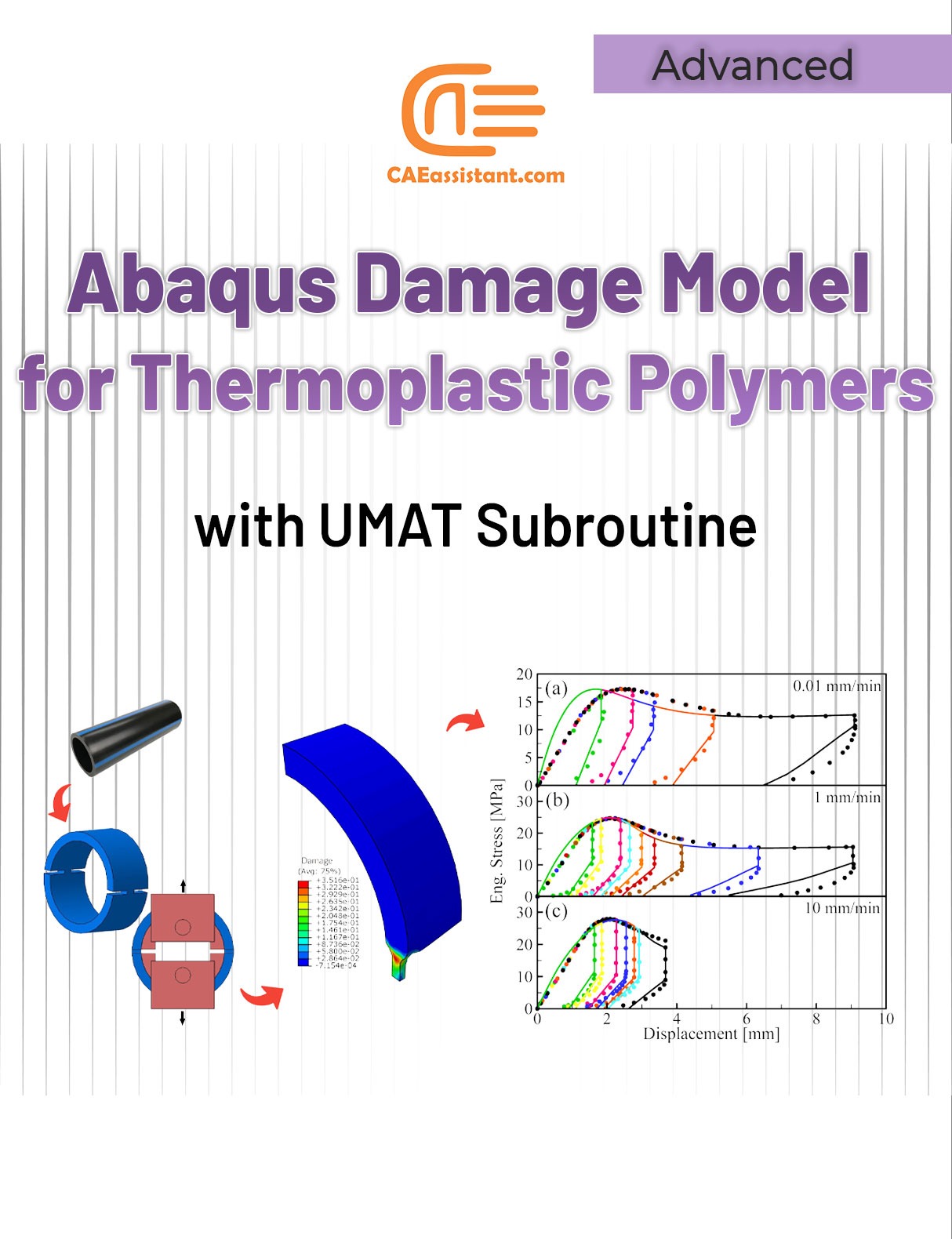
In this workshop, first, the geometry and test conditions such as the boundary condition and load are explained. Next, the modeling process is explained step by step. Finally, the simulation will be done, and the results will be discussed. In this example, there are three loading steps: loading, relaxing, and unloading. The results show that the model can simulate the time-dependent behavior of thermoplastic polymers precisely.

Moreover, the general description of how to write a subroutine is available in the article titled “Start Writing a Subroutine in Abaqus: Basics and Recommendations “. If you even do not familiar with the FORTRAN, you can learn the basics via this article: “Abaqus Fortran “Must-Knows” for Writing Subroutines”. You may also like this article to begin writing your own UMAT: “Start Writing Your First UMAT in Abaqus”.

It would be helpful to see Abaqus Documentation to understand how it would be hard to start an Abaqus simulation without any Abaqus tutorial. Moreover, if you need to get some info about the FEM, visit this article: “Introduction to Finite Element Method | Finite Element Analysis”. You don’t know which Abaqus software editions are suitable for you, Do not worry! This article would give you info about Abaqus editions: “How to download Abaqus? | Abaqus student & commercial edition” . One note, when you are simulating in Abaqus, be careful with the units of values you insert in Abaqus. Yes! Abaqus don’t have units but the values you enter must have consistent units. You can learn more about the system of units in Abaqus.